Introduction
|
|
Forcing files for the stream 2 scenarios:
They have been grouped into several directories
Historical 1860-2000 (First simulation):
These are the same forcing fields as used in the stream 1 IPCC simulations. Fore the core “stream 2” simulation only anthropogenic forcings should be used, without the solar and volcanic forcings, but with inclusion of the land-use changes represented by the fraction of crop and pasture derived by Nathalie de Noblet from the HYDE and Ramankutty and Foley (1999) databases.
This simulation will be used to start the 21-st century scenarios A1B-IPCC and A1B-450 .Historical 1860-2000 with natural forçings (Second simulation):
Same anthropogenic forcings as in the previous simulations, including land-use changes,with in addition the specification of solar and volcanic forcings as in stream 1.
This simulation is intended for allowing a better comparison with observed changes for validation purposes .
A1B IPCC simulation: (core simulation)
Here again the same forcings as in IPCC “stream 1” simulation derived from the SRES A1B marker scenariohave been gathered. In addition the land-use changes derived from the IMAGE A1B baseline scenario should be used.
The sulfate aerosol and ozone concentrations are the same as used in the stream 1 simulations.
Gridded emissions of SO2 on 1°x1° grid extracted from SRES for A1 scenario (zip file: SO2_Grids_A1.zip) (used by O. Boucher for computing sulfate concentrations)
A1B IMAGE simulation (Optional, though recommended, simulation):
All the forcing have been
derived from a new IMAGE simulation with the A1B hypothese.
A comparison of the A1-SRES with A1-IMAGE2.4/2007 has been made by
Detlef van Vuuren and Elke Stehfest in this document.
A1B 450 stabilization IMAGE simulation (core simulation)
The forcings have been derived from an new IMAGE simulation according to the A1B hypotheses but with the implementation of a stabilization policy to limit the forcing of GHG gases to be equivalent to that of a 450-ppm CO2 equivalent.
Short description of the new IMAGE scenarios:
The new scenarios have been implemented at Netherlands Environmental Assessment Agency (MNP) by Detlef Van Vuuren (Detlef.van.Vuuren@mnp.nl) and Elke Stehfest (Elke.Stehfest@mnp.nl) into the latest version of the IMAGE model, in which improvements have been made in the land use representation of the A1b scenario. This latest version of IMAGE has an updated estimate of carbon fertilisation in natural ecosystems, and reforestation has been added as a means to reduce emissions in order to meet the target of 450-ppm of CO2-equivalent. The data files include both the 450 ppm run and the baseline-A1b. The latter scenario is purely added for information (the A1b used by IMAGE is different from the A1b marker - but does comply to the standardisation criteria of SRES)
Some explanations can be found in this document.
For
more details on the IMAGE 2.4 model please consult the
MNP website: http://www.mnp.nl/image
.
A full description of the various components of IMAGE 2.4 is given in
the MNP publication:
Bouwman A. F., Kram T. & Klein_Goldewijk K. (eds.), 2006:
Integrated modelling of global environmental change. An overview of
IMAGE 2.4 (MNP Report no. 500110002, ISBN: 9069601516, Netherlands
Environmental Assessment Agency, Bilthoven, The Netherlands).
[pdf]
Applications to stabilisation scenarios are reported in:
van Vuuren, D.P.; M.G.J. den Elzen; P.L. Lucas; P. Eickhout; B.J.
Strengers; B. van Ruijven, S. Wonink; R van Houdt, 2007:
Stabilizing greenhouse gas concentrations at low levels: an
assessment of reduction strategies and costs. Climatic Change, 81,
119-159, doi:10.1007/s10584-006-9172-9
Output files from the new scenario:
As agreed upon, the global emissions and concentrations have been harmonized to 2000 values as they are available. For concentrations, the data that was provided on the RT2A site have been used. For emissions, all emissions have been harmonized to the mean of available inventories for 2000 emissions. A document indicates the values used in emission harmonisation (harmonization.doc ). The numbers differ somewhat from SRES (that guestimated in 1998 what 2000 emissions would be). Emission and concentration values were set to indicated values for 2000 using individual scaling factors. These scaling factors were assumed to linearly converge to 1 in 2100.
The results of the two new IMAGE simulations for global emissions and concentration have been provided as text files in zip files, a “legend.txt” explaining the content of these files. The same data are also given in excel spreadsheets.
The land cover maps are contained in two other zip files, with the land cover types indicated in an Excel file .
Excel files : A1B-450 A1B-baseline
Output zip files : A1B-450 A1B-baseline
Land cover maps : A1B-450 , A1B-baseline , land cover types
Crop fraction maps are also given for 19 crop types: A1B-450, A1B-baseline, crop types
Gridded emissions on a 0.5° x 0.5° grid for GHG and air pollutants have also been provided :
Maps:A1B-450 , A1B-baseline
Resulting
forcing fields
Crop and pasture annual
fractions:
Land-use data based on a combination of the crop dataset of
Ramankutty and Foley (1999), and pasture from the HYDE dataset
(Goldewijk, 2001) have been produced by Nathalie de Noblet (IPSL/LSCE)
to give a fraction of grid-cell covered by crop and pasture on a
0.5x0.5° global grid for each from 1700 to 1992.
The same method has been applied on the resulting land cover maps of a
former IMAGE scenario for A1B IPCC, and to the new IMAGE scenarios
A1B-450 and A1B baseline.
The recommended methodology is that each model keeps its vegetation map
as used in stream 1 simulations, and change only the crop and pasture
fraction as provided in this dataset. Nathalie has a number of python
scripts that could be used to interpolate the vegetation maps to
replace current crop and pasture areas for the preindustrial and has
offered to help the interested modelling groups (contact her at: Nathalie.de-noblet@cea.fr).
- The methodology for deriving the annual land-use fields for crop and
pasture is described in the report:
" Designing historical and future land-cover maps at the global scale
for climate studies", by Nathalie de Noblet-Ducoudré and
Jean-Yves
Peterschmitt [ pdf
]
- the land-use maps for cropland and pasture
fractions are available as NetCDF files at 0.5° resolution from
Nathalie de Noblet's DODS
server:
(A1B-450 ppm and A1B-baseline files are now usable, if you notice
problems please report them to Jean-François
Royer:Jean-francois.Royer@meteo.fr)
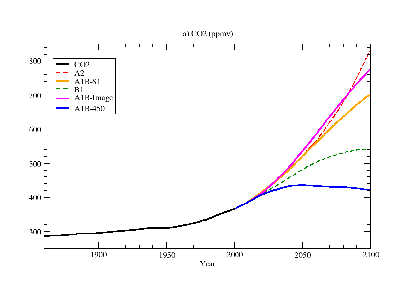
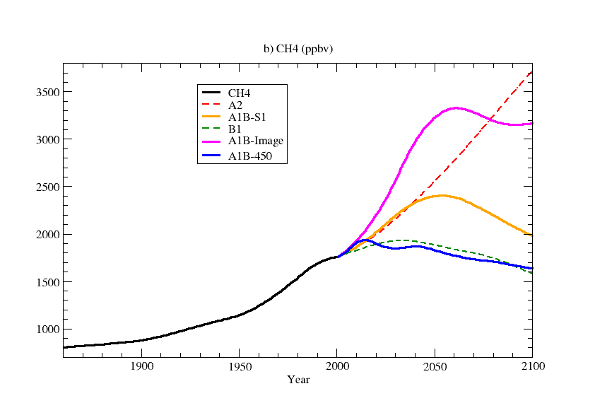
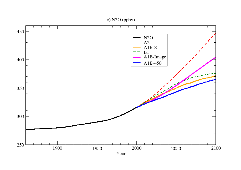
Greenhouse gas concentrations:
The series of CO2, CH4, N2O and CFC12 from the Excel files have been interpolated at annual resolution. The radiative forcing resulting from all the halogenated species except CFC12 has been converted into the CFC11 concentration giving the same radiative forcing. This has been done from the A1450.xls and baseline.xls files by adding the radiative forcings of “chloride”, “HFC”, “PFC&SF6” and “Halon” (columns E-H in sheet "forcing"), substracting the radiative forcing of CFC12 (computed from CFC12 concentrations from column C in sheet "Conc_clor" with a radiative forcing of 0.32 W/m2/ppb, a value taken from WMO/UNEP Scientific Assessment for Ozone Depletion 2002). The resulting forcing has then be reconverted back into CFC11 equivalent concentration called CFC11* using a radiative forcing coefficient of 0.25 W/m2/ppb. The annual series are contained in ascii files :A1B-450 and A1B-IMAGE.
Aerosol:
Using the emission
and concentrations from the IMAGE scenarios Olivier Boucher has used
a chemistry-transport model to derive new concentration of sulphate
aerosols for the A1B-450
simulations and A1B-baseline
.
The data files are password protected .
To
obtain login information please contact Annie
Rascol .
Other aerosol concentrations from IPCC SRES scenarios are also
available here.
Ozone:
Bjorg Rognerud has generated with the chemistry transport model of the University of Oslo maps of ozone concentrations for the end of 21st century for the new IMAGE A1B-baseline and A1B-450 scenarios. The ozone files are available from an ftp site .
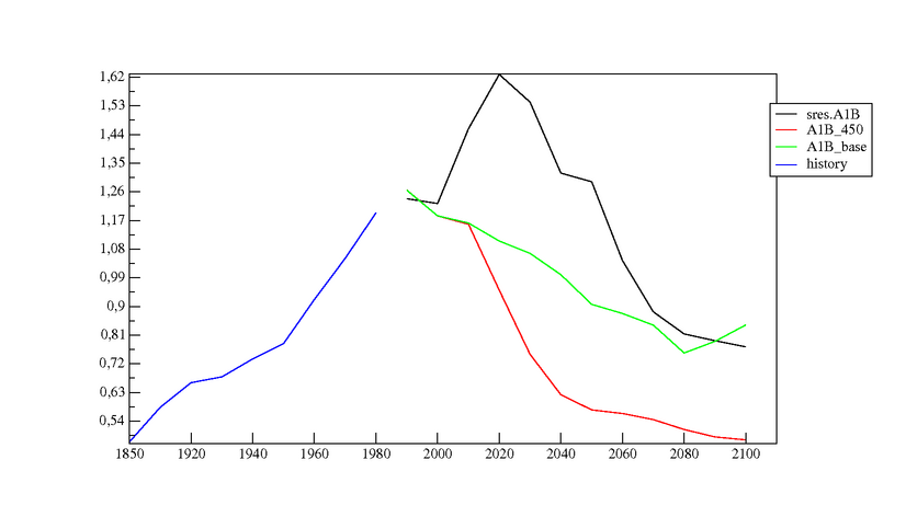
Comparison of the GHG concentrations and aerosol in the news scenarios:
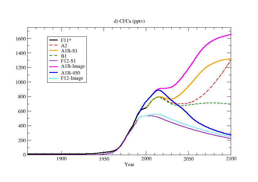
This figure shows the total sulfate aerosol with the Image A1B baseline scenario are much lower than in the SRES-A1B scenario used for the IPCC simulations (Stream 1) and still lower for the stabilisation scenario.