ALADIN Training NETwork
(ALATNET)
Contract n° HPRN-CT-1999-00057
Duration : 48 months
Second Annual Progress Report
March 2001 - February 2002
Scientific Network Coordinator :
Jean-François Geleyn
Météo-France, CNRM/GMAP
42, avenue Coriolis
F-31057 TOULOUSE CEDEX 01
tel. : 33 5 61 07 84 50
fax : 33 5 61 07 84 53
e-mail :
Jean-Francois.Geleyn@meteo.fr
Part A - Research Results
In the part concerning the non-hydrostatic dynamics, work
around the semi-implicit three-time-level semi-Lagrangian scheme evolved
towards the search for a more and more optimal choice of prognostic variables
(the experienced change in stability when modifying the choice of prognostic
variables is something that was unknown to be a specific feature of
non-hydrostatism) and this even led to a mixed prognostic-diagnostic solution
that gives a theoretical explanation for the (up to now) empirically justified
technique used in the Canadian model MC2. Further in this respect, the
iterative process that should lead to the two-time-level mirror version is
currently optimized and rationalised to become, if necessary, a competitive
solution for high-resolution modelling. Still in the same area of work the
problem of the lower-boundary condition in the semi-Lagrangian case has been
convincingly shown to depend on the way the vertical divergence is advected
(one should compute the divergence of the transported vertical velocity rather
than, like up to recently, do the operations in the inverse order).
For the ALADIN variational tools, the build of a solidly
justified prototype of high resolution 3d-var is quasi achieved with emphasis
on structure functions computed with the so-called "lagged" method
(i.e. concentrating on the scales that were not analysed by the model
providing the lateral boundary conditions) and on the use of "blending by
digital filter initialization" (a fully novel method for providing a
spin-up-free first guess at fine scale) to balance the high-resolution data
assimilation in a way that preserves most of the innovation coming from the
observations. There are however a few open questions concerning the best way
to take double nesting into account in such procedures and for the choice of
the most appropriate and/or economical way to do the blending step. Still in
this area, the work on specific features for the humidity analysis and land
surface assimilation (with a very advanced concept for 2d-var (time+vertical)
assimilation of surface prognostic variables over data dense areas) has
started to show good progress.
For high-resolution physics the prognostic treatment of
convective characteristics is achieved and emphasis has shifted to the other
potential prognostic variables : turbulent kinetic energy and condensates
(with first success for the so-called "functional boxes" approach
that tries to separate the issues of microphysics and of subgrid-scale cloud
formation into separate code entities). A new emphasis is also put on a more
in-depth rewriting of the input the convective parameterisation should deliver
to any microphysical parameterisation. The unexpected link between stable
boundary layer fluxes and cyclogenesis much downstream in the flux has been
confirmed with an improved and smoother parameterisation of the turbulent fluxes.
On a more case-to-case basis important progress was also
achieved in the following areas : snow evolution modelling and snow analysis,
further understanding of the respective roles of orography, time-stepping,
non-hydrostatism and horizontal resolution in the control of numerical noise,
comprehension of the reasons why the previous attempt to build a radiative
upper-boundary condition failed and role of the "regularised
physics" in TL/AD processes at high resolution. The latter step led to
the negative conclusion that 4d-var was unlikely to be a good solution per-se
for the life-time of the ALATNET programme and that it should therefore be
replaced as application target by 3d-var FGAT (first guess at appropriate
time). Sensitivity studies using the 4d-var basic tools should however be
further encouraged for longer term perspectives.
A.2. Joint Publications and Patents
Berre, L., G. Bölöni, R. Brozkova, V. Cassé, C. Fischer, J.-F. Geleyn, A. Horanyi, M. Rawindi, W. Sadiki and M. Siroka, 2002: Background error statistics in a high resolution limited area model. To appear in Proceedings of the HIRLAM Workshop on "Variational Data Assimilation and Remote Sensing", 21-23 January 2002, Helsinki, Finland.
Brozkova, R., D. Klaric, S. Ivatek-Sahdan, J.-F. Geleyn, V. Cassé, M. Siroka, G. Radnoti, M. Janousek, K. Stadlbacher and H. Seidl, 2001 : DFI blending: an alternative tool for preparation of the initial conditions for LAM. Research activities in atmospheric and oceanic modelling, Report N°31 of CAS/JSC Working Group on Numerical Experimentation , 1, 7-8.
Gospodinov, I., V. Spiridonov, P. Bénard and J.-F. Geleyn, 2002 : A refined semi-Lagrangian vertical trajectory scheme applied to a hydrostatic atmospheric model. Q. J. R. Meteorol. Soc. , 128, 323-336.
Siroka, M., G. Bölöni, R. Brozkova, A. Dziedzic, C. Fischer, J.-F. Geleyn, A. Horanyi, W. Sadiki and C. Soci, 2001 : Innovative developments for a 3D-Var analysis in a Limited Area Model: scale selection and blending cycle. Research activities in atmospheric and oceanic modelling, Report N°31 of CAS/JSC Working Group on Numerical Experimentation , 1, 53-54.
Soci, C., C. Fischer and A. Horanyi, 2001: Simplified physical parameterisation in the computation of the mesoscale sensitivities using ALADIN model. To appear in EWGLAM Newsletter, Proceedings of the 2001 EWGLAM/SRNWP meeting, 8-12 October 2001, Cracow, Poland.
Soci, C., A. Horanyi and C. Fischer, 2002: High resolution sensitivity studies using the adjoint of the ALADIN mesoscale numerical weather prediction model. Submitted to Idöjaras
Vivoda, J. and P. Bénard, 2001: Iterative implicit schemes for non-hydrostatic ALADIN. To appear in EWGLAM Newsletter , Proceedings of the 2001 EWGLAM/SRNWP meeting, 8-12 October 2001, Cracow, Poland.
Two more publications should be submitted soon to Mon.
Wea. Rev. :
Stability of the Leap-Frog Semi-Implicit Scheme for the Fully
Compressible System of Euler Equations. Part I: Flat-Terrain Case.
P. Bénard , J. Vivoda, P. Smolikova
Stability of the Leap-Frog Semi-Implicit Scheme for the Fully
Compressible System of Euler Equations. Part II: Case with Orography
P. Bénard, P. Smolikova, J. Masek
Only the new publications are mentioned here. The five research centres are involved in this list. The acknowlegment notice does not appear in extended abstracts, as for other grantings.
Part B - Comparison with the Joint Programme of Work
B.1. Research objectives
The programme of work is split in 12 main topics. Each partner is responsible for 1 to 4 topics, even if the basic work is shared between all teams. Let us recall the numbering of the involved research centres :
1 Toulouse(Fr) 2 Bruxelles(Be) 3 Prague(Cz) 4 Budapest(Hu) 5 Ljubljana(Si)
The thematic reports correspond to the revised work plan.
1. Theoretical aspects of non-hydrostatism
There is a nice progress in understanding the numerical
stability of the time schemes, as regards the integration of the fully
compressible equations of atmospheric motion. The stability properties were
found different for two-time-level and three-time-level semi-Lagrangian
schemes. In the two-time-level case a reasonable level of stability (robust
enough for potential numerical weather prediction use) can be achieved by
applying a predictor-corrector scheme, however three iterations of the
corrector step are necessary. Hence, the scheme is rather costly and ways on
"how to gain in efficiency while not destroying stability" are
explored. At the same time it was proven that an optimal choice of prognostic
variables enhances the stability of both two-time-level and three-time-level
schemes. New sets of prognostic variables were extensively tested and
validated. Another stabilizing factor is a decentering of the time scheme,
which has on the other hand strong damping properties. For this reason only
very gentle decentering factors can be used. A joint publication on the
stability issues is under preparation.
The second
main issue is the vertical discretization and formulation of the top and
bottom boundary conditions. There has been an intensive search on the problem
of spurious standing waves over the top of idealized mountains. The reason was
found and, indeed, it concerned the formulation of the semi-Lagrangian
advection of the prognostic variable describing vertical divergence. An
alternative approach for the vertical discretization of the vertical wind
component was proposed and successfully tested. A publication is also
envisaged. It remains to find the best way how to make this new approach fit
with the choice for the vertical wind implied by the above-mentioned new set
of prognostic variables.
A new non-reflecting upper boundary condition (RUBC), based
on recursive filtering, was considered. At first place the radiative (or
filtering) properties of RUBC were examined for gravity and acoustic waves
when their phase-speed is modified by a semi-implicit temporal scheme. Since
the radiative performance of RUBC depends on the phase-speed of waves to be
filtered, it was suggested that RUBC should be kept in an explicit form in
order to properly handle wave radiation. More conclusions can be expected from
2d and idealized 3d experiments, which will be carried on in the next period.
involved partners so far : P1, P3, P4
2. Case studies aspects of non-hydrostatism
As
an intermediate step between purely academic and real-case experiments, a
pseudo-academic study was performed in order to examine the stability criteria
for Eulerian and semi-Lagrangian advection schemes. The experimental setup was
academic but the orography faithfully reproduced that of Western Alps. As
mentioned, the aim of the study was to figure out at which resolution the
stability criteria for semi-Lagrangian advection schemes becomes more severe
than for the Eulerian one. The tests scanned a range of horizontal/vertical
resolutions from 10km/860m down to 1.25km/ 300m. It was found that the
semi-Lagrangian scheme does not meet earlier its stability limits and remains
competitive by enabling at least twice a longer time-step than the Eulerian
scheme. On the other hand other problems were confirmed as regards
semi-Lagrangian schemes, those solved at the theoretical level (topic 1).
Beside the pseudo-academic experiment a benchmark domain with an horizontal
resolution of 1km was created, for the area of Julian Alps.
For
the framework of full 3d experiments the IOP
(Intensive Observation
Periods) cases from MAP (Mesoscale Alpine Project) were chosen due to
the availability of additional observation data with high spatial and time
resolution. There are also some non-conventional additional measurements
available for that period (like wind profiler
data, aircraft measurements, etc...), useful in this frame of our work. The
main goal of this research is to
systematically evaluate the behaviour of high-resolution models. That is why
the decision has been taken to find the cases where already the
reference and coupling model (in our case ALADIN/LACE) is close enough to
reality (observed state). The main question we have to answer is what
additional quality can a model at high resolution bring and not why the
coupling model was wrong for some weather situation. The first target was to
compare non-hydrostatic to hydrostatic dynamics but it quickly turned out that
many other factors play a more important role. For this validation, the target
horizontal resolution of the ALADIN model was set to 2.5 km. In so high
resolution there is a great sensitivity to the representation of orography in
the model. The main outcome of the study of this problematic is that the use
of a "linear" truncation, together with a spectrally fitted and
coarser resolution (by a factor 1.5) orography provides a good basis for
running the model at very high resolution. With such an approach the
unrealistic wave patterns in the model outputs were significantly reduced. For
the current physics and dynamics, it seems that the problems identified in
very high resolution runs are more due to problems in dynamics than in
physics. The results also indicate great sensitivity to the jump of resolution
between coupling and coupled models. This will have to be investigated more in
detail in the work on the coupling problematics.
As
far as the orography itself is concerned, work has started on the definition
of a smoother transition than the brutal cut-off of the spectrum beyond that
of the so-called "quadratic" spectral truncation. Since the
elimination of the Gibbs feature over the sea areas calls for an off-line
minimisation in spectral space, the latter can be modified in order to
accommodate a smoother scale transition. Work on the method itself already
started and it was shown that the process can converge under a double
constraint. Generalisation to a lot of local sharp orography situations and
verification of the impact are the next steps to be considered.
involved partners so far : P1, P3, P5
3. Noise control in high resolution dynamics
Work on an alternative horizontal diffusion using the damping properties of semi-Lagrangian interpolators has been suspended for the time being but it is scheduled to restart in autumn 2002. The impact of decentering is still considered, as mentioned for topic 1, but with a low priority. Studies on the problem of orographic resonance stopped after some unsuccessful attempts, since the predictor/corrector approach (mentioned for topic 1) is expected to solve such problems.
involved partners so far : P1, P3, P5
4. Removal of the thin layer hypothesis
The work progressed in two directions, considering semi-Lagrangian advection and the ALADIN geometry.
involved partners so far : P1
5. Coupling and high resolution modes
§ Time-interpolation problem
A "phase-angle & amplitude" interpolation scheme was tested , instead of the traditional gridpoint interpolation. Test results on the "1999's Christmas storm" case were not satisfactory. Further studies and improvements of the method are expected. Meanwhile, during the first half of 2001 tests were performed in a 1d shallow-water model to compare the performance of different time-interpolation schemes for the coupling data. One scheme turned out to give better results than the other ones : the introduction of a second-order correction with an acceleration term. This type of correction was subsequently put in a broader context. In particular one could show that it can be seen as an extra term of a perturbation series. The practical consequence of this is that for such a series one can compute an estimate of the truncation error. The idea is then that this truncation error can be used to monitor the quality of the linear time-interpolation scheme.§ Spectral coupling
Spectral
coupling is a method of blending the large-scale spectral-state vector of the
coupled model so that the blended vector is equal to the large-scale one for
small wavenumbers and equal to the coupled one for large wavenumbers with
smooth transition in between. Spectral coupling is a perfect solution for
scale selection, but it does not take care about spurious waves : without
damping by the standard Davies' scheme, all waves that exit on one side of the
domain would freely enter on the opposite side.
Therefore the scheme can be considered only as a supplementary step of the
present Davies' scheme. It is expected to have the basic version of spectral
coupling ready in Ljubljana very soon. Some first results will then be
available on both the intrinsic performances of spectral coupling and on its
combination with the traditional (and probably retuned) Davies' coupling.
involved partners so far : P1, P2, P3, P4, P5
6. Specific coupling problems
§ Tendency coupling for surface pressure
The necessity of introducing a new formulation of coupling
for surface-pressure (ps) came up due to the strong impact of orography on ps.
Ps tendencies for coupling and coupled model are more connected than pure Ps
fields due to the differences in orographies. Ps-tendency coupling can be
formulated as a traditional Davies' coupling on ps plus a correction term.
That is why it was decided to follow this formulation in the code. Then the
original semi-implicit formulation of coupling remains unchanged and the
correction of the ps-tendency term can be introduced at the beginning of
time-step, explicitly in gridpoint space. State of the art : the code has been
developed, partially validated, but careful validation in a full 3d framework
is still to be done. The code is currently ported up to the newest model cycle.
§ Blending of fields
The preparation of the initial conditions by Digital Filter
Initialization (DFI) blending method was successfully implemented in the
operational ALADIN/LACE model, in Prague. Though the blending procedure is
used here without adding yet the observations, the improvements are noticeable
with respect to the previous dynamical adaptation method : better forecasting
skill, reduction of model spin-up. DFI-blending was further improved by
combination with incremental DFI in the forecast step (i.e. when the blending
increment to the previous ALADIN forecast is filtered, instead of the initial
blended fields). This is consistent with the intrinsically incremental
character of DFI-blending. The performance of DFI-blending was also confirmed
in the framework of the study of a MAP IOP case.
DFI-blending was also tried in double-nesting mode. However
differences with dynamical adaptation started to become quite small. To better
and tune the results in this special case, objective methods to analyse the
results (e.g. wavelets approach) and quantify the improvements at small scales
are now considered. Besides a detailed documentation was written. Work
concentrates now on the combination between DFI-blending and 3d-var analysis
(cf topic 11). The search for new, less expensive, blending methods is also considered.
involved partners so far : P1, P2, P3, P4
7. Reformulation of the physics-dynamics interface
Work recently restarted on two important topics for this branch of our activities. The first one concerns semi-Lagrangian advection (in the hydrostatic model for the time being) : where should the physical forcing be applied , i.e. at the origin of the trajectory like now (the most stable choice), in the middle (the most accurate choice) or at the end (the simplest solution) ? Second, in non-hydrostatic mode, which should be the partition the heating/cooling impact of diabatic changes between temperature and pressure evolutions ? The exact solution seems to be unnecessarily complex for the ALADIN present and targeted scales but a choice between the current trivial approximation (no pressure effect) and a more sophisticated intermediate choice is of interest to our research programme on non-hydrostatism.
involved partners so far : P1, P2
8. Adaptation of physics to higher resolution
§ Parameterisation of the small-scale features of convection
The
analysis of the properties of the convection scheme, started last year, was
pushed further, concentrating this time on the closure assumption. Two
modifications were made : following the wide-spread diagnostic that unresolved
precipitations had their proportion increased as the mesh size was reduced,
the dependency of the closure assumption on the mesh size was reintroduced in
the scheme, but together with the idea that water already used for resolved
precipitation is excluded from this balance. This required a retuning of the
characteristic length-scale for the closure (from 17 to 10 km). Furthermore,
thanks to the better balance between latent and sensible convective-transport
fluxes achieved last year, it became possible to make the
exclusion of the large-scale precipitation transparent with
respect to the moist enthalpy budget, a measure that stabilised and
rationalised the scheme.
Furthermore, two insufficient protections of the code against
"0/0" situations were identified and corrected. The steps
towards a more prognostic approach of the convection parameterisation are
described in the next section, mainly as a preparation of a unified
"convective+stratiform" input to microphysical calculations. The
parameterisation of suspended condensed phases, and the compatibility with
non-hydrostatic computations are still in the line of development but were
postponed owing to the above efforts, of higher priority.
§ Test, retuning and improvement of the various physical parameterisations in the framework of a very high resolution
The
effort on this part was relatively less important than last year and involved
mainly tests of the dependency of the convective closure-assumption on the
resolution. This work led on one side to the above-mentioned correction but on
the other side made previous efforts in the direction of case studies
irrelevant. Things only restarted recently in this direction (a fuller report
is therefore expected next year).
Some work was also performed on several cases of
hyper-activity of the model at high resolution but results are still divergent
from one case to the next and will thus need consolidation before being
transferred to effective and general measures to cure the problem.
§ Improved representation of boundary layer
The
work on the formulation of the exchange coefficients in the planetary boundary
layer (PBL) evolved from the stability's impact to the specification of the
so-called mixing-lengths. While a more general and situation-dependent
formulation is under development, an increase of the time- and
space-independent mixing lengths in the lower levels associated with a
decrease at the top of the atmosphere (i.e. a more clearly marked PBL) was
tested and became operational in Toulouse. Recent results in Prague indicate
that this retuning might have been exaggeratingly biased towards maritime
areas. In between, some inconsistencies in the original testing procedure were
traced-back and the effort will thus need some partial repeat.
The parameterisation of shallow convection was revisited on
the same occasion and two stabilising effects were obtained. The first one,
linked to the non-occurrence of shallow convection in the absence of
conditional instability, is now operational, while the second one, linking the
anti-fibrillation scheme to the prescription of the intensity of shallow
convection, still requires tuning, because of an imbalance on global moisture
budgets when the stabilising choice is implemented.
§ Improved representation of orographic effects
This part of the work received less attention than last year and was shifted towards the problem of "too much up-slope resolved precipitation and too little at the top" over mountainous regions (currently a problem for all high-resolution models). Several tracks have been identified but the coordinated work started only recently. Following the operational introduction in Toulouse of the so-called "linear grid" with "quadratic orography" for ARPEGE and ALADIN applications, work began on a smoother specification of the spectral removal of the highest modes of the observed topography, while still minimising as much as possible the Gibbs-effects over oceanic areas (cf topic 2).
involved partners so far : P1, P2, P3, P5
9. Design of new physical parameterisations
§ Implementation of a new parameterisation of turbulence
The theoretical bases of a new parameterisation based on the TKE (Turbulent kinetic Energy) approach were defined by Martin Gera in the framework of his Post-Doc study. More details are available in his report.
§ Use of liquid water and ice as prognostic variables, implementation of a new microphysics parameterisation
The treatment of cloud condensates by
prognostic variables required revisiting a series of earlier hypotheses about
the behaviour of the condensates in the model, particularly in the deep
convection scheme. Besides, a complete
re-organization of the convective package is on the way, as the package has to
play a new role in the forthcoming microphysics schemes : instead of producing
subgrid precipitation fluxes, it has to provide source terms in the
microphysics equations, in the form of convective fluxes of moisture, heat and
condensates. We propose a separate treatment of the
updraughts/downdraughts and "cloud-top evaporative instability",
after the computation of condensates and precipitation by the microphysical package.
In the frame of a high resolution LAM, no
complete solution appeared up to now in the literature to address the
possibility that the updraught occupies a significant part of the grid box. We
address this in two ways :
- taking into account the non-negligible
mesh fractions while computing the updraught profile and the updraught
contributions to large-scale tendencies;
- proposing a separate passing of the
updraught parcels through the microphysical package, as they could pass over
the microphysical thresholds (e.g. auto-conversion of condensate to
precipitation) well before the mean grid box parcels are considered.
The re-organization of the updraught routine
then includes : a new treatment of latent heats ; an explicit estimation of
condensate generation by the updraught ; the introduction of 3d updraught mesh
fractions ; a re-definition of the advected prognostic variables (advection of
the convective departure from the mean vertical velocity, instead of the
absolute updraught velocity) ; a new expression of the closure hypotheses ; a
modified computation of detrainment; a modification of the layer moisture and
heat budgets, which yield the convective fluxes instead of precipitation fluxes.
Parallely to this quite ambitious rewriting,
the more pragmatic approach of the so-called "functional
boxes" was pursued and a first nearly working package was obtained (the
last hurdle being the handling of a close 3 water-phases cycle around the
treble-point). It is now anticipated to include a microphysics
parameterisation of intermediate complexity in both approaches in order to
compare them, may be in the search for a future convergence.
§ New parameterisation of exchanges at sea and lake surface
These topics were left aside along the last year, since the involved researchers either left or were involved in more urgent tasks.
§ Improved representation of land surface, including the impact of vegetation and snow
A new description of snow cover was proposed and intensively
tested, with very promising results. It takes into account the mask effect of
vegetation and the time-evolution of the albedo of snow. Other approaches were
tested in parallel, but led to a poorer forecast skill than the present scheme.
Besides a set of newly available global high-resolution
databases for soil and vegetation was thoroughly checked and tested in
quasi-operational mode. But results were quite deceiving, with a negative
impact on global balances and equal or slightly worse scores in the comparison
to observations. A similar experiment was performed on the local scale,
testing a new database for soil texture over Hungary.
§ Refinements in the parameterisations of radiation and cloudiness
In the present radiation scheme the
integrated ozone profile is a function of pressure depending on 3 parameters,
and the same at each point of the model, which can be far from the reality. As
shown by the Romanian ALADIN team, a fit to correct climatological profiles
has a positive impact on forecasts. As a first step the UGAMP
climatology was used to fit the 3 parameters function. This kind of function
cannot adjust perfectly all the profiles, however the results are more closed
to the reality. Then 12 sets of 3 parameters fields were computed for ARPEGE.
An impact on the forecasts is shown by the first experiments. New experiments
will be necessary to estimate more precisely this impact.
It is planed to do a similar work on aerosol
profiles because they also have a strong interaction with the radiation scheme.
The single column studies done in the EUROpean Cloud Systems
context have shown that low levels ALADIN cloudiness is underestimated for
stratocumulus clouds, stratus or fogs. A new approach was developed, which
stands in two parts: (i) the cloudiness function uses the Xu and Randall
(1996) approach which produces greater cloudiness amounts for low clouds,
especially near grid-scale saturation with respect to the present operational
expression. (ii) the liquid water from shallow cumulus and from stratocumulus
is computed in a new form, which was designed following the work done on the
FIRE I stratocumulus case. This new approach leads to encouraging results on
the stratocumulus and fogs cases, and will be tested in d 3d more extensive
way in ARPEGE and ALADIN.
involved partners so far : P1, P2, P4, P5
10. Use of new observations
The initial working plan ( a. Yet unused SYNOP observations [0.;1.25], b. GPS and/or MSG observations [1.;3.], c. Doppler radar observations [2.25;4.], d. METOP (IASI) observations [3.;4.] ) was reconsidered in order to take into account both omitted but mandatory tasks and the effective availability of observations, and obtain a more realistic programme. It was decided to concentrate on a more extensive and accurate use of already available data, particularly on the following items :
§ An efficient quality control and selection procedure of observations for mesoscale LAMs
The screening procedure (i.e. the quality control and
geographical selection -thinning- of observations for 3d-var and also optimal
interpolation) for ALADIN has been updated and interfaced with ODB
("Observation Data Base", the new tool for observation management
just upstream the model). A procedure to build specific databases, containing
only observations in the ALADIN domain, was designed and the corresponding
documentation written.
The problem of thinning of AIREP (aircraft) and SATOB
(satellite) data, over the ALADIN/France domain was examined afterwards.
AIREPs provide informations on wind and temperature, with a large dispersion
in space (mainly around / between airports) and time (with a peak in the
afternoon). With the operational horizontal thinning distance in ARPEGE, 170
km, most data are
rejected. Experiments with decreasing lengths, down to 10
km, were performed. The main
improvement is obtained between 25 and 10
km. An impact on 3d-var analysis increments is noticed in the
upper troposphere and the stratosphere for wind, in the boundary layer and the
stratosphere for temperature. This study enabled to underline a problem
induced by the handling of AIREPs in screening, plane by plane independently.
Observations valid at the same point but not at the same time, so quite
different, are kept as input for 3d-var analysis. This fosters the march
towards more continuous data assimilation systems (4d-var, or 3d-var at a
higher frequency, or any intermediate solution).
Problems are different for SATOBs. Thinning must be performed
in 2 steps, but observations are far less, and used only over sea. So the
proposed reduction of the thinning distance is smaller.
The next steps will be the improvement of the management of
boundary-layer observations, the introduction of new data, and the
introduction of more controls.
§ A more extensive and accurate use of conventional data (surface observations, soundings and aircrafts informations)
The use of more dense (in time and space) or new (e.g. snow
depth) surface (SYNOP) observations was first addressed within applications
based on optimal interpolation. The first studies addressing upperair analysis
started along the last year. Three points were addressed. The impact of using
denser aircraft data is described in the previous section.
The second one concerned the use of a precise horizontal
positioning of the radio-sounding balloons, instead of assuming that the
balloon climbs purely vertically. The monitoring of corrected/completed
sounding-bulletins (TEMPs) proved there could be a small positive effect when
considering the horizontal drift. However, this technique is not yet ready for
a wide use since the balloon horizontal coordinates, though known, are not
coded in TEMPs; a change of standards would be necessary.
The third study focussed on the use of screen-level humidity
observations in the upperair analysis (usually not considered in global data
assimilation systems). It aimed at checking which are the shape and amplitude
of the increments when using mesoscale background-error structure functions.
In this case the increments keep small and local.
The priority is now to improve vertical interpolations in the
boundary layer within observation operators (i.e. when computing the
equivalent of the observed data from model fields).
§ A more extensive and accurate use of available satellite data
GPS and MSG observations must be forgotten, since they won't
be fully available before the end of the present project.
The work on IASI data has started, in the framework of an
ALATNET PhD study (Malgorzata Szczech). IASI data are routinely assimilated by
global NWP models, but used only over sea where a very simple
observation-operator may be derived. But LAMs mainly covered continental
areas, where the parameterisation of emissivity is far more complicated.
The use of ATOVS data is also considered, with two directions
of work. The first studies addressed the use of "local" information,
provided by EUMETSAT or the satellite teams of some NMSs (as France or
Hungary). These datasets have only a local coverage, but are denser and
available sooner than those delivered by the WMO network. Which is completely
in line with the main features of data assimilation in mesoscale LAMs.
Experiments performed with ARPEGE 4d-var showed a positive impact. The second
priority is the use of raw data. The required developments are starting.
§ The progressive use of some non-conventional data, particularly radar reflectivities
Such observations are very likely to be managed using two
procedures successively. As a first (and expected quick) step, they will be
used as "pseudo-observations", i.e. controlled and converted, using
informations from the model, into standard observation types. The second step
is the design of the corresponding observation operators.
A first detailed case study using such pseudo-observations in
3d-var analysis is underway. The data consist of pseudo-profiles of relative
humidity, obtained from MeteoSat imagery via a cloud classification (to
identify the saturated areas, and their height) associated with radar
information (especially to identify mis-specified low and deep clouds).
A small team specialized on radar observations should be
set-up at the end of 2002. However progress in this domain will highly depend
on the state of research on micro-physics and precipitations.
involved partners so far : P1, P3, P4
11. 3d-var analysis and variational applications
§ Introduction
The 3d-var related activities of the ALATNET project continued on the solid basis of the first year's results and on the increased manpower. Three ALATNET centres were basically involved in the work : Toulouse, Prague and Budapest, with more recent contributions from Bruxelles. The subject of the second ALATNET seminar was data assimilation and this fact further drew attention to that part of research. The position opened in Budapest was successfully filled for the second part of the year, which also helped. Last year's progress is summarised hereafter, following the subtopics identified in the ALATNET working plan.
§ Definition and calculation of new background error statistics, impact of domain resolution and extension, identification of horizontal relevant scales
At the beginning of the reporting period there was a general
agreement on the use of the lagged-NMC method to compute background-error
statistics for ALADIN 3d-var. It was proved best for analysing only the
smaller scales in the limited-area model (LAM), the large-scale corrections
being provided by the coupling data assimilation system.
More evaluation studies were required however. First the
spectra of differences between ARPEGE and ALADIN forecasts valid for the same
dates and ranges were computed, in order to evaluate the respective
contributions of (initial) model differences and forecast to large and small
scales. This compares well with the result of the lagged-NMC method.
Second its suitability to the case of nested LAMs was
examined, using the ALADIN/HU model (coupled to ALADIN/LACE with a resolution
ratio of 1.5 only). The sensitivity of the lagged-NMC method to the forecast
lengths and the forecast differences was evaluated, computing and comparing 28
different types of statistics and subsequent single-observation experiments.
The main preliminary conclusion of this work is that the lagged method is much
less effective in double-nested environment, especially when the resolution
ratio between coupling and coupled models is small. Particularly the reduction
of the error variances at large scales induced by the lagged-NMC method also
affects the smaller ones here. This can be attributed to the fact that the
driving model has a strong influence on the results through the lateral
boundary conditions.
Refinements are already studied. The geographical variability
of background-error statistics was analysed, addressing the impact of latitude
first. It was shown it is possible to introduce such a dependency in the
formulation of the background cost-function using a simple block-diagonal
matrix. This work is now extended to longitudinal variability and a new
formulation of Jb. Besides other approaches are under evaluation : wavelet
methods for representing spatial variations of error covariances, Analysis
Ensemble Method in the framework of the PhD study of Margarida Belo Pereira.
§ Scientific investigation of the problem of extension and coupling zone, analysis of the impact of initialization
The main motivation for dealing with the problem of the
extension and coupling zones was to avoid analysis signals penetrating
(through the purely mathematical extension zone) the opposite side of the
domain. This artefact was observed in the first single-observation
experiments. A few remedies were tested, but the solution came from another
research direction. It appeared that lagged-NMC statistics allow for an
acceptable reduction of the analysis increments throughout the extension zone.
On the other hand, the use of standard-NMC statistics can produce quite
unrealistic analysis fields, even with a large number of observations well
inside the computational domain.
The question of initialization was heavily investigated and
tested. It strongly interacts with the use of DFI-blending, the formulation of
the background term and the coupling strategy. Standard (applied on model
fields) and incremental (applied on analysis increments) digital filter
initialization (DFI) procedures were considered. The results may be summarised
as follow :
- cycling without DFI-blending : standard DFI is mandatory
both inside the assimilation cycle and for the subsequent forecasts ;
- cycles with DFI-blending : incremental DFI or no DFI at all
do have almost the same impact, so the need for initialization is still
unclear; standard DFI has a very negative effect on analysis increments, and
should therefore be avoided if possible.
Both results are obtained using lagged-NMC statistics.
Experiments performed with standard-NMC statistics didn't include blending and
required classical initialization. The fact that standard DFI is not needed
after a DFI-blending cycle indicates that most of the structures that are
filtered out must be driven by large- or medium-scale structures, with some
forcing from the coupling. The actual effect of incremental DFI will be
further investigated. Especially, it is not clear whether the small benefit
observed over the first 3 hours actually leads to a meteorological improvement.
§ Management of observations in 3d-var from academic single-observation experiments to use of any available data
Single-observation experiments were widely used in order to
check the applied background-error statistics and the structure functions of
the 3d-var scheme. The tests also proved the robustness of the scheme.
When the results of the single-observation experiments proved
satisfactory then full-observation experiments started. The standard set of
observations are surface measurements, radiosonde vertical profiles, flight
reports, etc ... The procedure of selection, particularly the definition of
the optimal density, of observations was adapted to ALADIN (cf topic 10).
Experiments showed that the basic available observations are sufficient for
basic 3d-var validation. However the increase of the amount and diversity of
observations would be surely beneficial for the performance of the
assimilation scheme. A first case study using a wider range of observations
was initiated recently (cf topic 10).
§ Coupling problems in variational data assimilation, interaction with blending
The
combination of DFI-blending with 3d-var was extensively tested. Three basic
strategies were compared: Blendvar (3d-var analysis after DFI-blending),
Varblend (blending after 3d-var) and classical 3d-var (when the first guess is
a 6-hour forecast and standard background-error statistics are used). In the
first two cases lagged background-error statistics were used, in agreement
with the application of the (basically incremental) blending algorithm. Tests
were performed either over long periods, looking at the mean skill, and over 2
well-documented cases.
Tests over long periods revealed the importance of the
coupling fields to be used at the initial time in the framework of classical
3d-var. Here one has to choose between space-consistent (i.e. using analysed
fields) and time-consistent (i.e. issued from a forecast) coupling. The
experimentation proved that in case of combination with blending
time-consistent coupling should be used and for the classical strategy (now
considered as an obsolete option) the space-consistent coupling is the right procedure.
Case studies demonstrated the improvement brought by
DFI-blending and lagged-NMC statistics (but not to which extent each) to the
balance between mass and wind. Blending provides a balanced combination of
large- and small-scale analysis increments, while lagged statistics allow a
good control of noise (preventing from gridpoint storm triggering) thanks to
its mesoscale length-scales and balances. The first specific case study was
performed on the situation with strong convection developing along a frontal
limit. The second case was the same MAP IOP one used for tests of the
DFI-blending alone. For the first time there was a case where clearly each
step (DFI-blending and 3d-var) improved the forecast ...
§ Intensive scientific validation and improvement of 3d-var
The main objective of the validation is to find the best
scientific strategy to exploit the 3d-var data assimilation scheme in an
operational context. Lot of experiments were already run in Prague, Budapest
and Toulouse (to mention only ALATNET centres), to answer the remaining open
questions. The following main ingredients were or remain to be tested:
- Combination with blending (which cycling, which type of blending),
- Initialization (standard, incremental, no),
- Background-error statistics (standard, lagged, which
integration lengths and time-shifts),
- Coupling (time-consistent, space-consistent),
- Nesting.
The degree of freedom is rather large and the optimal choice
is likely to depend on the characteristics of the model where 3d-var is going
to be applied. The results of all the experiments were evaluated having a
subjective look on the obtained analysed and forecasted fields, computating
simple objective scores, scrutinizing the time evolution of different fields
at different locations and examining energy spectra, at least for two-week
long experiments. Validation was more careful for case sudies, such as the MAP
IOP 14 experiment. Here the validation used independent MAP observations,
about precipitations (land-based and radar reflectivities), satellite pictures
(water vapour, SSMI)
As main conclusions, the strong beneficial impact of the
blending step, with its injection of fresh large scale conditions, has been
shown. The 3d-var analysis of conventional data has only a secondary (yet
apparently positive) impact. The role of initialization is not fully
understood, as described previously. The most spectacular success of the
Blendvar cycling lies in its ability to reproduce some of the mesoscale
features that were absent from the operational forecasts, while clearly seen
on the observations. Also, an overall more active and time-consistent
evolution of the precipitations is noticed.
§ Development of variational type applications
Significant work was dedicated to the sensitivity studies,
where the main issue was to see how the forecasts of the model can be improved
by the modification of initial conditions. These initial conditions can be for
example changed by adding a scaled gradient provided by the sensitivity
fields. A major step forward was that also the effect of physics in the
sensitivity patterns were examined. The conclusions are far from being final,
but it can be already said that there is a potential to use the gradient
(sensitivity) patterns for improving the initial conditions. All the dynamical
understanding of the potential improvements helps in the future development of
the 4d-var scheme. Furthermore this effort included refinements of regular
physics for use in ALADIN.
Another application is the computation of singular vectors,
where the first experiments with the full model were performed. The obtained
results until now are very preliminary, however the investigations should
continue especially taken into account the possible predictability activities
around the ALADIN model (where singular vectors might serve as hints of
dynamically relevant perturbations in the initial condition of the model).
An original use of variational tools is a-posteriori
diagnostics for the tuning of background-error standard deviations (and more
generally data assimilation systems). As a general principle, one compares the
actual value of a diagnostic, and compares it with the theoretical value. The
difference indicates a first-order correction to be applied to the standard
deviations. So it has been shown that this tuning does indeed work in the
desired fashion when a time series of diagnostics is considered. A more
sophisticated method, also tested on global model data, has however failed to
give any stable results. A detailed documentation on this approach was written.
§ Summary
The activities around the 3d-var scheme of the ALADIN model are in line with the working plan, therefore it is expected that for the next year the operational implementation of the scheme will be possible. The work on variational type of applications started and will be continued until the end of the project providing valuable hints for the implementation of the 4d-var scheme for the ALADIN model.
involved partners so far : P1, P2, P3, P4
12. 4d-var assimilation
Several
results (mainly but not exclusively obtained in the ARPEGE operational
framework for 4d-var at Météo-France) forced us to reconsider
the strategy of the ALATNET research plan on this topic :
- Fictitious
rainfall above desert areas was traced back to the misuse by the minimization
algorithms of the degrees of freedom linking geopotential thicknesses and
moisture contents (and the problem may extend to spoilt initial fields for
temperature too) ;
- The
algorithm for part of regularized physics (boundary layer
processes) became unstable in its TL/AD (tangent linear / adjoint) runs when
the time-step was increased in length following the adoption of a
semi-Lagrangian perturbation algorithm ;
- ALADIN
tests of sensitivity to initial conditions were seriously degraded by a
similar instability, linked this time to the parameterization of large-scale precipitation.
It is
anticipated that similar or even worse problems will appear at high resolution.
The search for solutions has started, focusing on large
scales first to solve operational problems. But the results of these studies
and their further validation at small scales are still uncertain. The initial
target is thus severely compromised.
Research around continuous data assimilation systems will go
on, but the main objective is transferred from 4d-var to 3d-FGAT (first guess
at appropriate time). This newly proposed technique is an intermediate between
3d and 4d variational assimilations, where the time dimension is considered in
the comparison between forecasted and observed fields.
involved partners so far : P1
Some more details may be found in the ALATNET Newsletters, available on the ALATNET Web-site : http://www.cnrm.meteo.fr/alatnet/ .
B.2. Research method
There is no change to mention here.
B.3. Work Plan
The completion of the work plan was discussed and the initial program adjusted during the fourth official meeting of the ALATNET steering committee (Budapest, 8 March 2002).
Breakdown of tasks
Part of the initial work plan must be adjusted since :
- some topics are now of limited interest : for instance 3a-b will be solved by 1 and 3c;The partition of work among partners did not change, apart from an increased contribution of the Hungarian team to the work on coupling.
Schedule and Milestones
Changes in the schedule are detailed in the thematic reports
and hereabove. The milestones have again to be modified, to take into account
the emergence of new alternatives and the present delays.
The main steps forward along the first two years are compared
to the initial and revised schedules in the table below :
Dates |
Initial and revised milestones |
Progress of the project (main steps) |
01-03-00 Start of the project |
§ First training course
· Prototype version of the 2d-version achieved · Analytical study of orographic resonance, tests · Preliminary design of predictor/corrector scheme · Search for new time-interpolation methods for lateral boundary conditions, or new coupling scheme · Analytical study for relaxing thin layer hypothesis · Test of new descriptions of sea and lake surfaces | |
01-06-00 |
¨ Start of 3 PhD & 1
Post-Doc studies
· Scale-selection strategy for 3d-var defined | |
01-09-00 |
¨ Start of 1 PhD study
· First results on orographic forcing at small scales | |
01-12-00 |
· Identification of stability
problems in semi-implicit NH
· Framework for high resolution validation available; first tests · Improvement of the 1d-version for the validation of new developments in physics · Prototype version of 3d-var + blending · Starting validation of the singular vectors computation | |
01-03-01 1st annual report |
¨ Start of 1 Post-Doc study
· First proposals for new NH variables · Operational version of blending | |
01-06-01 |
=> reference HR NH
version ready
+ 3d-var analysis ready + first set of observation operators ready -> reference HR NH
version ready
|
§ Second training course
¨ Start of 2 PhD studies · Prototype version for coupling the surface pressure tendency · New prognostic convection scheme available |
01-09-01 |
¨ Start of 2 PhD & 1
Post-Doc studies
· New proposals for NH variables · Starting the design of new validation tools for high resolution · Major changes in description of boundary layer · First sensitivity studies with 3d-var | |
01-12-01 |
¨ Start of 1 PhD study
· Restart of the work on the upper boundary condition · New snow parameterisation ready · Starting an in-depth update of radiation scheme · Starting work on new observation types and on the use of "standard" observations at high resolution · Revised targets for new observation types · Simplified physics tested at small scales using variational tools | |
01-03-02 Mid-term review |
=> reference HR NH
version fully validated with improved coupling
+ prototype version of 4d-var ready -> reference HR NH
version fully validated with improved coupling & physics
|
· "Functional boxes" approach for handling liquid water and ice working |
The future milestones may be summarized as :
· After three years :Research effort of the participants
The situation has slightly improved when compared to last year, but the total research effort of the participants is still a little below the initial estimation as shown in Table 1.
For the young researchers, the problem is due to the late recruitments in Budapest (P4), Ljubljana (P5) and Bruxelles (P2), but the situation is safe now.
For the background effort the situation is very contrasted. Toulouse (P1) and Prague (P2) are beyond the target, but a bit favoured through the organization of the respective ALATNET training courses, in Gourdon and Radostovice respectively. Bruxelles and Budapest are below, but on a good way. The situation is very difficult for Ljubljana, especially since the recent reorganization / takeover of HMIS, as explained in part B.6 .
Table 1 : Professional research effort on the network project after 2 years (person-months)
Participant |
|||||||||
targeted |
realized |
rate |
targeted |
realized |
rate |
targeted |
realized |
rate | |
1 2 3 4 5 |
51 19 27 14 17 |
31½ 13 30 10 16 |
0.62 0.68 1.11 0.71 0.94 |
147 70 77 55 73 |
192½ 44 79½ 41¼ 14 |
1.31 0.63 1.03 0.75 0.19 |
198 89 104 69 90 |
224 57 109½ 51¼ 30 |
1.13 0.64 1.05 0.74 0.33 |
Totals |
128 |
100½ |
0.79 |
422 |
371¼ |
0.88 |
550 |
471¾ |
0.86 |
This problem and an in-depth analysis of the potential of each partner to catch-up with the initial targets within the remaining two years of the contract led to the following proposal for a redistribution of the target background effort. The French team (relatively at ease) will take over part of the effort of its Belgian (at its limits) and Slovenian (unlikely to reach a target now too high for its new situation) partners. The part of the Hungarian team is slightly reduced to keep its total effort unchanged (after last year modifications of the Young Researcher programme), and the same procedure is applied to Slovenia. The impact of the proposed shifts (P1 +65, P2 -22, P5 -43 / P4 -4, P5 -3) and that of the change in recruitments made last year are described in Table 2. The initial and present targets for the total effort, including all researchers, don't differ (1055 person-months).
Table 2 : Professional research effort on the network project (person-months / individuals)
Participant |
|||||||||
initial |
final |
so far |
initial |
final |
so far |
initial |
final |
so far | |
1 2 3 4 5 |
78 38 46 24 38 |
78 38 46 28 41 |
31½ 13 30 10 16 |
283 136 173 106 133 |
348 114 173 102 87 |
192½ 44 79½ 41¼ 14 |
17 9 12 7 7 |
17 9 12 7 7 |
20 7 9 8 5 |
Totals |
224 |
231 |
100½ |
831 |
824 |
371¼ |
52 |
52 |
48 |
The modified target efforts are in bold characters.
B.4. Organisation and Management
B.4.1 Description
The description provided in the first annual report is still
valid. An ALATNET Web-site was created and is updated regularly :
http://www.cnrm.meteo.fr/alatnet/.
It provides informations on ALATNET events, young researchers,
coordinators, research plan, training courses, ... and is linked to the
Web-sites of the European Commission and of the ALADIN project (hence to the
web pages of ALATNET partners). A specific ALATNET e-mail list was created for
exchanges between students, mentors, and coordinators :
alatnet@meteo.fr.
Students may also use the other ALADIN e-mail lists of course.
An ALATNET Newsletter is published every 6 months, jointly
with the ALADIN Newsletter. There is a clear distinction between contributions
but they are edited together, to provide the young researchers an overview of
the more general research around ALADIN and to make their results known by a
large scientific community. The Newsletters are available on the ALATNET and
ALADIN Web-sites and sent to all ALADIN partners and to each of the five
European SRNWP coordinators.
The Young Researchers had (and will have) the opportunity to
meet other young scientists during the open 3 ALATNET training courses. All of
them attended or will attend an ALADIN or a wider European workshop during
their employment (roughly such a travel every 10 months), and as far as
possible present their work there. The participation is detailed in part
B.5.4 .
B.4.2 Major network meetings and workshops
§ Second official meeting of the ALATNET steering committee : § Third official meeting of the
ALATNET steering committee :
- Paris (Fr), 31 Mai 2001
-
problems encountered so far, preparing the selection of Young Researchers, ...
§ Fourth
official meeting of the ALATNET steering committee :
-
Budapest (Hu), 8 March 2002
-
preparation of the Mid-term Review, revision of the work plan, ...
§ Mid-term Review of ALATNET (1
EU representative, 1 Expert, 12 Y.R., 8 supervisors) :
-
Bruxelles (Be), 22/23 April 2002
Except for the very recent Mid-term Review, the corresponding reports, as well as an historical account of the project life, are available on the ALATNET Web-site.
B.4.3 Networking
§ Short visits between research centres along the second year (on ALATNET fundings or not, excluding the pure participations to the second ALATNET training course) :
* Toulouse ==> Bruxelles
|
D. Giard , |
19/03/2001 |
: coordination |
|
P. Pottier , |
19/03/2001 |
: coordination |
|
J.F. Geleyn , |
05/07/2001 - 06/07/2001 |
: coordination |
|
J.F. Geleyn , |
30/08/2001 - 31/08/2001 |
: convection |
|
J.F. Geleyn , |
31/10/2001 |
: coordination |
|
J.F. Geleyn , |
03/02/2002 - 05/02/2002 |
: orography |
* Toulouse ==> Prague
|
J.F. Geleyn , |
13/03/2001 - 18/03/2001 |
: coordination |
Toulouse ==> Budapest
Toulouse ==> Ljubljana
* Bruxelles ==> Toulouse
|
P. Termonia, |
03/03/2001 - 10/03/2001 |
: coupling |
|
L. Gérard, |
06/06/2001 - 09/06/2001 |
: coordination |
|
A. Deckmyn, |
06/06/2001 - 23/06/2001 |
: coordination (+ training course) |
|
I. Gospodinov, |
05/06/2001 - 23/06/2001 |
: coordination (+ training course) |
|
P. Termonia, |
06/06/2001 - 23/06/2001 |
: coordination (+ training course) |
|
O. Latinne, |
16/11/2001 - 23/12/2001 |
: new soil & vegetation description |
Bruxelles ==> Prague
Bruxelles ==> Budapest
Bruxelles ==> Ljubljana
* Prague ==> Toulouse
|
R. Brozkova , |
01/01/2001 - 15/01/2001 |
: non-hydrostatic dynamics |
|
P. Smolikova, |
01/02/2001 - 31/03/2001 |
: non-hydrostatic dynamics |
|
R. Brozkova, |
06/06/2001 - 24/06/2001 |
: coordination (+ training course) |
|
A. Trojakova, |
15/10/2001 - 12/12/2001 |
: non-hydrostatic dynamics |
|
M. Janousek, |
01/12/2001 - 15/12/2001 |
: geometry + non-hydrostatic dynamics |
|
M. Janousek, |
11/02/2002 - 15/03/2002 |
: non-hydrostatic dynamics |
* Prague ==> Bruxelles
|
M. Janousek , |
19/03/2001 |
: coordination |
Prague ==> Budapest
Prague ==> Ljubljana
* Budapest ==> Toulouse
|
R.Randriamampianina |
17/04/2001 - 17/08/2001 |
: ATOVS observations |
|
A. Horanyi , |
22/05/2001 - 23/06/2001 |
: coordination (+ training course) |
|
S. Kertesz, |
06/06/2001 - 06/07/2001 |
: 3d-var & observations (+ training course) |
|
S. Kertesz, |
01/09/2001 - 31/10/2001 |
: 3d-var & observations |
|
R.Randriamampianina |
09/09/2001 - 30/09/2001 |
: ATOVS observations (+ training course) |
|
G. Radnoti, |
08/12/2001 - 13/12/2001 |
: coupling, coordination |
* Budapest ==> Bruxelles
|
A. Horanyi , |
19/03/2001 |
: coordination |
* Budapest ==> Prague
|
T. Szabo , |
12/03/2001 - 21/04/2001 |
: coupling |
|
G. Boloni, |
15/10/2001 - 23/11/2001 |
: 3d-var & blending |
|
H. Toth, |
26/11/2001 - 21/12/2001 |
: parameterization of radiation |
Budapest ==> Ljubljana
* Ljubljana ==> Toulouse
|
J. Merse, |
22/04/2001 - 20/06/2001 |
: cloudiness parameter. (+ training course) |
|
N. Pristov, |
06/06/2001 - 20/06/2001 |
: coordination (+ training course) |
|
K. Stadlbacher, |
06/06/2001 - 20/06/2001 |
: coordination (+ training course) |
|
J. Jerman, |
09/06/2001 - 20/06/2001 |
: coordination (+ training course) |
|
J. Jerman, |
08/12/2001 - 14/12/2001 |
: coordination |
|
J. Roskar, |
08/12/2001 - 14/12/2001 |
: coordination |
* Ljubljana ==> Bruxelles
|
J. Jerman , |
19/03/2001 |
: coordination |
* Ljubljana ==> Prague
|
J. Jerman, |
02/04/2001 - 15/04/2001 |
: high resolution modelling |
|
K. Stadlabacher, |
13/05/2001 - 17/05/2001 |
: high resolution modelling |
|
D. Cemas , |
21/05/2001 - 09/06/2001 |
: high resolution modelling |
|
D. Cemas , |
13/08/2001 - 31/08/2001 |
: high resolution modelling |
Ljubljana ==> Budapest
§ Invitations on ALATNET fundings concerning European non-ALATNET countries
* in Bruxelles : Doina Banciu (Romania), 17-23/03/2001 (work on convection with Luc Gérard)
§ Discussions between involved scientists during European workshops :
* 10th ALADIN workshop on Scientific developments (Toulouse, Fr, 07-08/06/2001),* 23rd EWGLAM & 8th SRNWP
workshops (Cracow, Pl, 08-12/10/2001),
with the participation of :
D. Giard, P. Pottier, M. Szczech (P1),
R. Brozkova, C. Smith, J. Vivoda (P3),
A. Horanyi, C. Soci (P4),
N. Pristov (P5)
§ Additional distant supervision of young researchers between ALATNET centres :
J.F. Geleyn (Fr) >> L. Gérard (Be) (till summer 2001 : PhD defense)§ Regular e-mail exchanges between contact points for each topic in ALATNET centres : as usual.
B.5. Training
B.5.1 Publicity for vacancies
For each call, vacancies were published on the Web-site of the E.C. and a notice was sent to each European ALADIN partner, and to SRNWP coordinators who are responsible for broadcasting informations to other European NMSs. The publicity to universities was left to individual NMSs.
B.5.2 Progress in recruitment
§ First call for candidacies :
- publication : 19 April 2000§ Second call for candidacies :
- publication : 26 December 2000§ Third call for candidacies :
- publication : 30 March 2001B.5.3 Integration of young researchers
Given
the standing structure of the ALADIN action, the experience already acquired
in Toulouse and Prague for structured visits, the past benefits of the
bilateral Slovenian-French and Hungarian-Slovenian actions and the experience
of the recruited Post-doc students, there was no particular surprise in the
integration of all twelve Young Researchers, especially the seven new ones, in
their teams. Administrative difficulties from the host countries were however
still noticeable in Bruxelles.
B.5.4 Training of young researchers
§ Individual training of young researchers
The basic training of young researchers :§ Participation to European workshops
- C. Smith, C. Soci, M. Szczech and J. Vivoda attended the
joint "European Working Group on Limited Area Modelling" &
"Short Range Numerical Weather Prediction" (EWGLAM/SRNWP) networks
annual meeting in Cracow (2001);
- C. Smith and J. Vivoda attended the SRNWP specialised workshop on Numerical Techniques in Bratislava (2001);
- G. Balsamo attended the SRNWP specialised workshop on "Surface Processes, Turbulence and Mountain Effects" in Madrid (2001);
- K. Stadlbacher attended the World Meteorological Organisation workshop on "Quantitative Precipitation Forecast Verification" in Prague (2001);
- G. Balsamo and C. Soci could attend the 2000 EWGLAM/SRNWP meeting on the spot in Toulouse;
- M. Szczech participated to the Ecole d'été internationale "Interactions Aerosols - Nuages - Rayonnement" in La Londe des Maures in 2001 and, in 2002, S. Alexandru should participate to a NATO school on Data Assimilation;
- I. Gospodinov, C. Soci, M. Szczech and K. Stadlbacher attended the 10th ALADIN workshop in Toulouse (2001).
§ ALATNET training courses
The ALATNET program of work includes the organization of 3
training courses covering the main aspects of Numerical Weather Prediction
(NWP) :
- on High
Resolution Modelling (Radostovice, Cz, 15-26/05/2000) ,
- on Data
Assimilation (Gourdon, Fr, 11-22/06/2001) ,
- on Numerical
Techniques (Kranjska Gora, Si, 27-31/05/2002) .
These seminars are open to European students and to
non-European ALADIN students. All European NMSs are informed in due time, as
for ALATNET vacancies. The ALATNET young researchers have to attend this
advanced training (once employed of course).
B.5.5 Special measures to promote equal opportunities
For the third and last call for candidacies, the following partition of (selected) candidates was obtained :
Recruitments / Candidates for the third call | ||||
Pre-Doc |
Post-Doc | |||
Country |
Women |
Men |
Women |
Men |
ALADIN (*) |
4 / 5 |
1 / 3 |
0 / 0 |
1 / 1 |
non ALADIN |
0 / 1 |
0 / 1 |
0 / 0 |
0 / 0 |
(*) There were no candidates from ALATNET countries, though allowed for this call.
This leads to the following parity among Young Researchers :
Young researchers | ||||
Pre-Doc |
Post-Doc | |||
Country |
Women |
Men |
Women |
Men |
ALADIN (*) |
4 |
4 |
0 |
2 |
non ALADIN |
0 |
1 |
0 |
1 |
We managed to reach the ratio of 1/3 of women among the Young
Researchers (without any cheating !), which is slightly more than the
equivalent partition within the ALADIN project (with huge discrepancies
between teams).
Despite our good-willingness only 2 Young Researchers come
from other European NWP consortia.
The parity women / men was also preserved in the participation to the second ALATNET training seminar. Two non-ALATNET students came from non-ALADIN countries (Finland and Mexico). A few Italian students registered but finally cancelled their travel. There was no selection, of course.
Involved Countries |
Parity |
Second Training Course | ||
Students |
Mixed |
Teachers | ||
|
ALATNET (with young researchers) |
Women |
6 |
1 |
3 |
Men |
12 |
4 |
8 | |
|
European , ALADIN , non-ALATNET |
Women |
6 |
2 |
0 |
Men |
5 |
0 |
0 | |
|
European , non-ALADIN |
Women |
1 |
0 |
0 |
Men |
0 |
0 |
0 | |
|
non-European , ALADIN |
Women |
0 |
1 |
0 |
Men |
1 |
0 |
0 | |
|
non-European , non-ALADIN |
Women |
1 |
0 |
0 |
Men |
0 |
0 |
0 | |
|
total contribution |
Women |
14 |
4 |
3 |
Men |
18 |
4 |
8 | |
Retrospectively,
8 ALATNET Young Researchers attended the Radostovice Seminar of 2000 prior to
their recruitment in the Network. For the Gourdon Seminar, all 6 already
recruited Young Researchers attended, and one of the participants was a just
selected candidate for the last round of recruitment. Nearly all Young
Researchers shall attend the Kranjska Gora Seminar.
B.5.6 Measures taken to exploit multi-disciplinarity in the training program
This part of the ALATNET programme is indistinguishable from the global effort to make the ALADIN project a real link between training, research and operational aspects of Numerical Weather Prediction, a multi-disciplinary theme in itself (fluid dynamics, atmospheric physics, signal processing, numerical analysis, optimal control, behaviour of stochastic systems, interface with computing techniques, ...). A few numbers are probably sufficient to explain how structured is this part of the environment of the ALATNET effort: more than 30 equivalent-persons, between 1 and 2 PhD per year, 35% of the effort realised through research-training stays outside the 15 home institutions, this corresponding to 13% of the total cost of the project (salaries and computing-costs included).
On
a two-year average, the ALATNET-bound effort (directly and indirectly
financed) represents 42% of the scientific ALADIN activity (for 6% of the
direct financing, all activities included: training, research, computing and
telecom). The presence of the Young Researchers increases to 48% (from the
above-mentioned 35) the rate ofvisit-type work in the ALATNET activity.
B.5.7 Connections to industrial and commercial enterprises in the training program
NWP activities are a rather internal business since they encompass their own "industry" (i.e. the production of daily operational weather forecasts, mainly for public service aims and for regulated aeronautical forecast procedures) and one more striking figure of the ALADIN project is the existence of 14 (pre-)operational versions. This mixed research/operational environment thus offers a good opportunity for witnessing the transfer process from research to daily application (and its specific problems), even if the Young Researchers are not directly participating in this part of the NWP effort. The link with computer manufacturers is also important in such a "simulation bound" scientific activity.
B.6. Difficulties
The former
Hydro-Meteorological Institute of Slovenia (as ALATNET Centre in Slovenia) was
merged into the Environmental Agency of Republic of Slovenia (EARS) in the
middle of 2001. The EARS as successor of HMIS became the governing institution
for ALATNET in Slovenia. The transition between the two institutions was
smooth as far the administrative part of the ALATNET project is concerned but,
owing to the former leave of Dr. Mark Zagar to a post-doc position in Sweden
and to the reorganization of HMIS, the number of persons working in numerical
weather prediction, especially on research aspects and correspondingly on the
ALATNET research topics, is now significantly decreased. The work related to ALATNET is now evidently
even more connected with the research stays of PhD students in Ljubljana. It
is agreed with the management of the EARS that the number of people working
locally on ALATNET should increase so we may hope some improvement.
Jure Jerman is now the official ALATNET coordinator for Slovenia.
Part C - Summary Reports by Young Researchers
Scientific strategy for the implementation of a 3d-var data assimilation scheme
for a double nested limited area model
Progress
The purpose of the work is to find the best scientific strategy for the implementation of the 3d-var data assimilation scheme for a double-nested limited area model. ALADIN/HU is a double-nested limited area model which is coupled to ALADIN/LACE, itself coupled to ARPEGE. The boundary conditions are obtained from ALADIN/LACE integration, at 12 km resolution. The resolution of the ALADIN/HU model is about 8 km.
To produce a good forecast, a good description of the initial conditions is necessary. The objective of data assimilation is to define the best initial state of the model taking into account all the possible information. 3d-var consists in minimizing a cost function, in order to get the best fit to the available information sources. The cost function is the sum of three terms : J=Jo+Jb+Jc where Jo represents the departures from the observations, Jb represents the departures from the first-guess, and Jc controls the amplitude of gravity waves in the analysis. At the moment for ALADIN model only the first two terms are defined.
In 2000, the 3d-var data assimilation scheme was ported to Budapest for the Origin 2000 machine of the Hungarian Meteorological Service. The AL13 version of ALADIN model is used for 3d-var, taking into account classical NMC statistics for the background term (Parrish and Derber, 1992), and only SYNOP and TEMP observations for the observational term of the cost function. The first-guess is the 6 h forecast from an earlier model run. It contains information on the small scales (the scales of the model) but, being a forecast, it is not fully precise. The 3d-var scheme is running four times per day, but the subsequent 48 h integration is performed twice per day.
The steps performed in the 3d-var scheme are : first the preparation of the observational data, then the distribution of the observational data across the available processors, followed by a screening procedure which calculates the high resolution departures and makes the quality control of the observations, then the incremental variational analysis is performed, using the first-guess (6 h forecast from the previous model run), the observation file prepared by the screening, and the classical background error statistics file. Because the 3d-var data assimilation scheme is acting for the upperair meteorological fields, after the variational analysis step, the optimal interpolation analysis is applied for the surface variables, and finally the model integration is realized to obtain the next first-guess (Siroka and Horanyi, 1999).
The verification is made to evaluate the model performance. The statistical measures (rmse - root mean square error -, bias) are used as indicators of the extent at which model prediction match observations. These objective scores are calculated for the forecast of the model using 3d-var scheme, and also for the operational forecast (using the dynamical adaptation). The compared fields are the temperature, the geopotential, the zonal and meridional wind, the relative humidity, the direction and intensity of the wind, at different pressure levels. The first results indicate that the scores are better for the wind, temperature and geopotential, using 3d-var scheme. The worst scores are for the relative humidity (Alexandru, 2002).
Trying to understand the behaviour of the humidity field, we performed many experiments, using the operational coupling files, and some coupling files prepared in Prague (from the ARPEGE and ALADIN/LACE assimilation cycles). As a reference for all the experiments, we were running the model in dynamical adaptation. For the experiments with 3d-var scheme we decided to use different coupling techniques, with and without incremental digital-filter initialization (DFI) in cycling and to obtain the first-guess from the ALADIN/LACE files prepared in Prague.
The problem with the humidity appeared again. So we chose a case when the scores of the humidity using 3d-var scheme were bad compared with the forecast of the model using dynamical adaptation. For this case, we rerun all the experiments for 6 h integration without DFI in production. Then we used the humidity treated as univariate variable. Another idea was that maybe the analysis coming from the ALADIN/LACE model is so closed by the first-guess, that even if the 3d-var scheme realizes some features of the small scales, they are too small. So we tried to have the first-guess using the ARPEGE files. But the results of the humidity didn't show an improvement.
In all these experiments, the humidity field seems to be better represented using dynamical adaptation than the 3d-var scheme, which is quite an unexpected result. Now we concentrate on checking whether all the procedures are working correctly, and understanding the results for the humidity field.
Perspectives
After we'll resolve the humidity problem, we decided to focus our attention on the next aspects:
a) Case studies. For the beginning we choose two cases. One case is from the period for which Gergö Boloni made the tests with "Blendvar" and "Varblend" (combinations of 3d-var analysis and blending of spectral fields) in Prague (Boloni, 2001), and the idea was to see the results for a double nested limited area model. Both cases were chosen because we considered them as interesting meteorological situations, with a front passing through the domain. On these cases we will make the experiments with the different background error statistics (standard, lagged), first-guess fields (the 6 h forecast of the previous run, blending of the ALADIN forecast with ARPEGE analysis (Giard, 2001)), initialization methods, together with their a-posteriori evaluation, etc ...
b) We want to establish which one of the coupling techniques is better.
c) Then we plan to run four times per day the spectral blending procedure for the first-guess. The necessary files, which contain the large scales are provided from Prague.
d) Other experiments will be performed using the "Blendvar" and "Varblend" combinations, with the lagged statistics.
Future work
The next months will be devoted to the experiments with the different background error statistics, first-guess, initialization methods and posteriori evaluation. So at the end of this first stay, we would like to get an idea about the best possible version of a 3d-var data assimilation scheme for a double nested limited area model.
Future training activities
In May 2002 I will participate to a seminar on "Data Assimilation for the Earth System", organized by the NATO Advanced Study Institute (ASI). In autumn 2002 I shall attend for the EWGLAM (European Working Group on Limited Area Modelling) meeting, to be held in Netherlands.
References:
- D. Parrish and J. Derber, 1992: "The National Meteorological Center's spectral statistical interpolation analysis system". Mon. Wea. Rev., 120, 1747-1763.Assimilation of soil moisture from screen-level variables: test of 2D-var
and OI techniques
with ALADIN NWP model.
Introduction
The soil moisture content of continental areas enters into the hydrological cycle and energetic balance as a major importance parameter. The reservoir of water stored in the soil is generally available for vegetation and could be released in the atmosphere through the evapotranspiration process and later redistributed to the soil by the precipitations. The soil moisture content regulates the partition between latent and sensible heat flux at the surface affecting a large number of boundary-layer and low-troposphere processes. An accurate estimate of this quantity over extensive areas might provide opportunities for many applications and for this reason agricultural, hydrological, meteorological and climatological studies have considered the subject in recent research.
The assimilation of screen-layer observations for soil moisture correction is here considered for study. The operational assimilation of soil moisture performed at Météo-France on the global scale (within ARPEGE), based on the "optimum interpolation" (OI) technique, is tested within a mesoscale model (ALADIN). A variational assimilation technique is implemented to analyse the soil moisture by assimilating 2 m data of temperature and relative humidity. We consider 2d (z and t) variational approach, under the assumption of horizontal decoupling of surface processes between gridpoints. This hypothesis is firstly put forward considering the small scale involved in the soil processes, far from the actual grid mesh in numerical weather prediction (NWP) : few meters versus a few km. A validation test is then designed to evaluate the influence of neighbour gridpoints (Figure 1). Thus, the method is applied on every grid point singularly and the gain matrix is directly computed given the small dimension of the problem. The variational technique keeps count of the full physics of the model and therefore the corrections applied on the control variable are adapted to the current meteorological conditions and the gridpoint characteristics (texture, vegetation properties, and the previous soil state).
The 2D-var and the OI test on a 6-hour time window
The sequential assimilation by means of the 2D-var and OI techniques is performed on selected cases. The observation departures are computed at the synoptic time (00, 06, 12, 18 h UTC). The variational approach is based on a linear estimation of the observation operator H, obtained by applying a perturbation to the control variable W, the mean soil moisture. The 6-hour sequential assimilation cycle allows to focus on specific features and permits the comparison of the analysis corrections. The higher resolution observational network present over the ALADIN domain allows to chose a smaller forecast-error correlation-length for both 2 m temperature and relative humidity; therefore in the analysis it is reduced from the 300 km used in ARPEGE to 100 km for ALADIN.
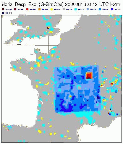
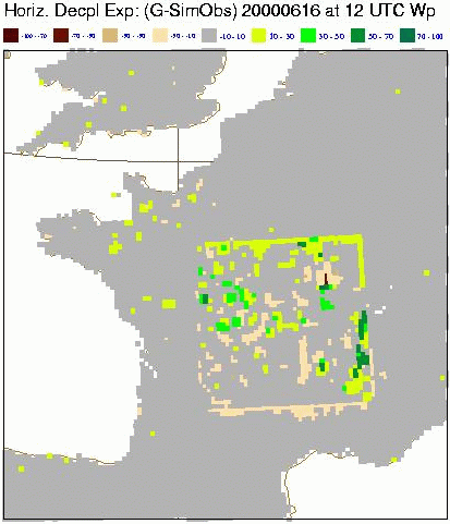
Figure 1 : Validation of horizontal decoupling between gridpoints. Test performed on the 16th June 2000 at 12 h UTC. A reference initialization of the mean soil moisture content (W) at 6 h UTC is used to generate simulated observations. The initial soil moisture is then modified and the span between the reference state and the modified state (Wmod - Wref, in mm) is shown in figure (a). Figures (b) and (c) report the errors on temperature and relative humidity at 2 m obtained after 6 hour integration with respect to the simulated observations (innovation vector that is used for the soil moisture analysis). The residual error after the analysis done at 12 h UTC (W analysis -Wref , in mm) is given in (d)
The variational test is performed on the same cases in order to tune the background error covariance for the mean soil moisture. The equivalent of the OI coefficients are extracted from the elements of the gain matrix K (Figure 2). The masks of non-sensitive zones in both methods highlight the same macro areas in the domain. The masking technique in the OI is based on physical thresholds reached by the guess for certain fields, that activate the masking. The 2D-var masking is performed on thresholds for the perturbation effects. Although the mask procedure is on-off type, the transitions between analysed areas and masked areas are less sharp with the variational method. The structure of the coefficients is studied in diurnal and nocturnal phases to see the variation in magnitude. Different dates are also taken to see the seasonal influence.
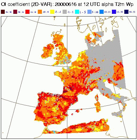
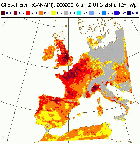
Figure 2 : (a) The gain matrix K obtained from the 2D-var method compared with (b) OI coefficients for 2 m temperature on the16 June 2000 at 12 h UTC. In the presented case the OI coefficient for temperature is structured in magnitude larger from South to North according to the increasing vegetation cover over Europe for the selected days. The equivalent 2D-var coefficient has an opposite structure according to stronger radiation fluxes toward the South. This is also consistent with latent heat exchange at the surface boundary-layer and therefore with a stronger correlation between soil and near-surface atmosphere.
The set-up of background-error covariance for the mean soil moisture is 15 % of the reference soil moisture range, between the field capacity and the wilting point. This rather large value for the error covariance matches the magnitude of corrections applied by the OI method and it is therefore maintained for a matter of comparison. An operational context should consider a more realistic value of about 5 % of this reference range. The perturbation of the guess has been chosen as 20 % after tuning.
Assimilation tests
Two parallel assimilation tests are done over 15 days of spring (4-18 June 2000) using a 6-hour sequential analysis. Both experiments are initialised with a medium soil moisture. This rather crude start allows to study the formation of horizontal gradients in soil moisture during the assimilation cycle. The initial smooth fields of soil moisture reach articulated structure in few days of assimilation. The corrections are of the order of a few mm during the night hours and a few tens of mm during day time, for both methods. The OI method tends to create larger wet and dry areas, the 2D-var creates different patterns, less large and pronounced and of relative smaller scale. After three days of assimilation the two methods lead to two different patterns where only some peaks of dry and wet zones match. An off-line soil moisture field, produced with the ISBA-MODCOU coupled model, is also tested in order evaluate the benefits of a more realistic initialization. In fact, the achievement of a realistic soil moisture content does not necessarily lead to an improvement of the forecast. A strong readjustment of soil moisture, even if unrealistic, can compensate model biases in a 2 m forecast. Hence, four different soil moisture initializations for the 16 June 2000 have been compared. The common macro structures are preserved. Scattered wet-dry peaks are more evident in the OI-ARPEGE cycle as probably related to the cumulated effect of continuous operational cycle. The ALADIN OI and 2D-var seem to produce coherent structures, drying the southern and the eastern parts of Europe and particularly the Iberian peninsula, and moistening the Alpine region and Massif Central over France according to climatological considerations and as figured out by the ISBA-MODCOU original data.
A set of forecasts initialised with the 4 soil moisture fields are evaluated in the case study 13-18 June 2000. The operational ARPEGE forecast interpolated to the ALADIN resolution is used as reference. The computation of bias and rmse scores put in evidence a diurnal cycle as main signal, common to every forecast with the different initializations. Improvements and deteriorations of the forecast with respect to the operational OI-ARPEGE are observed for every initialization. The 2D-var analysed mean soil moisture shows an overall positive impact during diurnal hours and reduces deterioration with respect to the other initialisations at night. Validation on an extensive period and further tuning of the method are needed to assess the positive impact.
Conclusions and perspectives
The use of a linearized variational technique for the mean soil water content analysis from 2 m simulated observations and for different time-windows has been evaluated. The results are promising and further tests are necessary to validate the method with real observations. Particularly interesting is the 6 hour time-window as it allows comparison with the OI method. The study of the H matrix highlights several features related to synoptic situations. The mask of non-sensitive zones allows to further improve the convergence towards the reference state. The dynamically derived coefficients of correction provided by the variational method are compared to the statistical OI coefficients used operationally. Independent assimilation-cycle tests have been set in order to compare the abilities of both methods for soil-moisture assimilation on the mesoscale.
The OI method highlights that strong corrections of mean soil moisture are performed during the 6 h sequential assimilation.
Although uncertainties remain on the spatial and temporal evolutions of water in the soil, the use of a more realistic soil moisture should be pursued also by means of improvements of the surface schemes. A realistic state will allow a closer interaction of meteorological and other applications. The implemented 2D-var method has shown capability to converge to reference state and the first tests give encouraging results for mesoscale assimilation of land-surface soil moisture content. The simplicity and portability of this method make it a possible instrument to evaluate the impact of new observations (i.e. satellite data) on different mesoscale NWP models.
In the near future the method will be tested on other soil variables. The optimization of the variational method will be pursued testing different assimilation windows (24/48 hours) and increasing the density of observations (in space and time). A set of parameters difficult to tune, as thermal conductivity or hydraulic coefficients, may be also considered for study.
References
Balsamo G., Bouyssel F., Noilhan J., 2002 - "Mesoscale variational assimilation for land surface variables". SRNWP/HIRLAM Workshop on surface processes, turbulence and montain effects - INM- Madrid 22-24 October 2001List of Visits during ALATNET research period:
Madrid (Spain)- 22-24 October 2001 - SRNWP/HIRLAM Workshop on
Surface Processes, Turbulence and Mountain Effects.
Achievements: In this scientific context I could
experience the highly active environment of a workshop and have the occasion
to personally meet several authors of the publications I have been based on
for my research. Different approaches dedicated to surface processes modelling
has been presented and raised questions and ideas. The work I have presented
has been positively commented and considered and I could benefit of many
advises and suggestions from the working group, helpful for the prosecution of
the research.
Gourdon (France) - 11-22 June 2001 - ALATNET Seminar on Data Assimilation.
Achievements: This two weeks seminar offered a great
tool for data assimilation work. The subject has been introduced and
extensively treated and many related research topics with their actual
challenges have been also presented.
Toulouse (France) - 24-26 October 2000 VPP Supercomputing
course - TotalView - MPI basics.
Achievements: Basis of supercomputing facilities on
Fujitsu VPP5000 have been presented together with debugging tools. Exercises
and examples helped the understanding.
Toulouse (France) - 9-13 October 2000 - 22nd EWGLAM meeting
(with MAP session) / 7th SRNWP meeting / 2nd EUCOS meeting.
Achievements: Attendance to these European joint
meetings has been interesting. The state of the art of research and
operational applications for several NWP groups in Europe was presented.
List of publications during ALATNET research period:
"Mesoscale variational assimilation for land surface
variables" - Workshop Report - Madrid (Spain)- 22-24 October 2001 -
SRNWP/HIRLAM Workshop on Surface Processes, Turbulence and Mountain Effects.
Report for ALATNET Newsletter 3, November 2001
Report for ALATNET Newsletter 2, February 2001
Report for ALATNET Newsletter 1, August 2000
Improving the assimilation of water in a NWP model
Introduction
The time integration of numerical weather prediction (NWP) models requires the knowledge of the initial state of the atmosphere. Moreover it is known that the forecasts from NWP models are very sensitive to small errors in the initial state. The aim of the meteorological data assimilation is to determine this initial state, trying to make it as close as possible to the true state of the atmosphere. However, the observations are not perfect and are insufficient to describe the atmospheric state. Therefore, a short range (6 hours) forecast (known as background) is used as a preliminary estimate of the true state. So, the analysis field is a combination of background and observations. The weights given to observations and to background are determined by the magnitudes of errors at each location (variances) and of the correlations between errors at different locations (covariances). The matrix which contains these statistics for the background is known as the B matrix. Nevertheless, both background and observation errors can only be estimated since the true state is not known. In summary, the task of a data assimilation system is to find out the weights that minimize the uncertainties in the analysis fields using both the background and the observations.
The first goal of this study is to learn more about the specific humidity errors features in the background and its connections with errors in others variables. In order to accomplish that, the Analysis Ensemble Method was "implemented" into the 3d-var analysis in ARPEGE. Another goal of this study will be the improvement of the assimilation of Special Sensor Microwave Imager (SSM/I) radiances, using the knowledge acquired during this study about the structure functions of the background errors of specific humidity.
Analysis Ensemble Method
The purpose of this method is to estimate the background error statistics. In this method an ensemble of independent analysis experiments is performed. For each experiment (member) and for each analysis cycle, all observations are perturbed adding an independent random number, which has a Gaussian distribution with mean zero and variance equal to the prescribed variance of observation error. These perturbations will create a perturbed analysis for each member. The differences between the perturbed analyses of different members are a measure of the uncertainties in the analysis. Afterwards, a 6 h integration of the numerical model is performed, using the perturbed analysis. So, in this way the uncertainties in the analysis fields are propagated to the 6 h forecast and consequently to the next analysis cycle, in the form of uncertainties in the background. After a few days of assimilation, the statistics of the differences between background fields for pairs of members of the ensemble equilibrate and it is assumed that the differences between the 6 h forecasts of independent members of the ensemble represent the background errors, from which the statistics related to the B matrix can be estimated.
Description of the experiments
The ensemble consists of 10 31-level 3d-var analysis experiments for the period of 1-30 May 2001. Initial conditions for all experiments were provided by an analysis for 18 h UTC of 30 April from a 3d-var unperturbed experiment.
The independent analysis members were arbitrarily numbered from 31 to 40. The differences between the 6 h forecast valid at 12 h UTC for consecutively numbered members were calculated between 4/5/2001 and 30/5/2001. This provided 9x27=243 differences between background fields, from which we estimate the statistics of the background error.
Moreover, the differences between members were computed also for 12 h UTC analysis and for both 6 h and 12 h forecasts valid at 18 h UTC. The aim of these experiments is to study the relation between the uncertainties in the background and in the analysed fields, as well as its impact on the next 6 h forecast.
Results: preliminary study of some statistics
The results show that most of the variance of divergence and vorticity errors near tropopause and at stratospheric levels comes from synoptic scales, for wavenumbers between 20 and 40. For middle and low troposphere the spectra are much broader, which means that contributions from mesoscale phenomena are also important.
The maximum variance of the specific humidity (q) errors occurs for wavenumbers between 15 and 25. Moreover, the contribution from mesoscale to the variance of q error is smaller than for divergence. In Planetary Boundary Layer (PBL), the maximum variance of temperature error comes from wavenumbers between 10 and 30. For levels above PBL, the largest uncertainties in temperature field comes from the planetary and synoptic scales, i.e. wavenumbers less than 10. Moreover, for levels below 500 hPa, the uncertainties in temperature and in specific humidity are larger for analysis than for background.
On average, most of the variance of the background errors for mean-sea-level pressure (mslp) comes from planetary and synoptic scales (wavenumbers less then 14). Moreover the analysis at 12 h UTC is able to reduce significantly the background errors of mslp, mainly in the planetary scales. The errors of mslp and temperature in the 6 h forecast valid at 18 h UTC are smaller than the errors in the 12h forecast valid at same hour. This result is due the reduction of the uncertainties in mslp caused by the 12 h UTC analysis. In the middle and upper troposphere the analysis of temperature contributes also for this result. However, for specific humidity in low troposphere, the uncertainties in the 12 h forecast valid at 18 h UTC are larger than in the 6 h forecast valid at same time. This result means that contrarily to the case of temperature, the reduction on the mslp uncertainties produced by the analysis are insufficient to create a positive impact in the 6 h forecast valid at 18 h UTC for specific humidity. Possibly, this can be explained by the more complex coupling between q and mslp, comparing with the coupling between temperature and mslp.
Results: visualization of forecast and analysis differences
In order to learn more about the results given by the statistics, the differences between two members were studied individually for analyses and forecasts, for few days. As an illustration of the impact of the uncertainties pattern of the analysis on the forecasts, the time evolution of the differences between members 36 and 37 over Europe are shown for day 6.
On Europe region, the uncertainties on the analysis of mslp are smaller than on the background, with some exceptions (like Sweden and North of British Islands). Moreover, this has a very positive impact in the mslp 6 h forecast valid at 18 h UTC, except over Centre and South regions of Italy, where the errors of the 12 h forecast are smaller than the 6 h forecast valid at same time (figure 1).
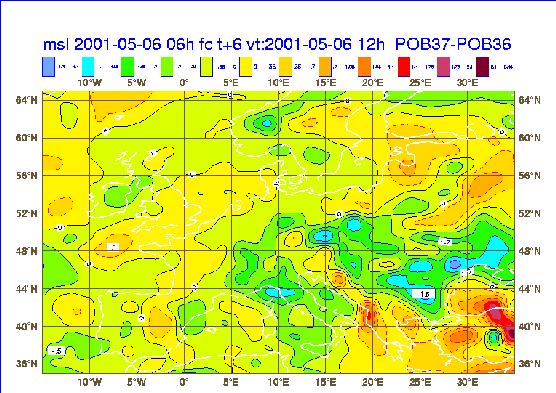
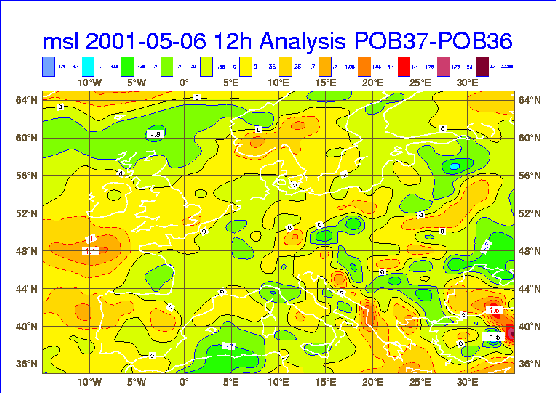
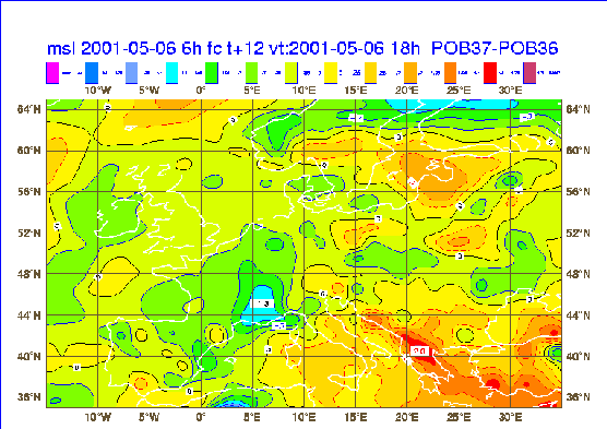
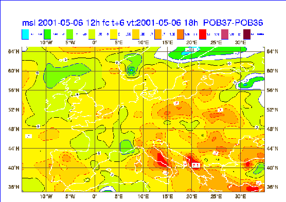
Figure 1 : Mean sea level pressure differences (isolines of 0.35 hPa) between member 37 and member 36, for 6 h forecast valid at 12 h UTC (superior left), for analysis (superior right), for 12 h forecast (inferior left) and for 6 h forecast (inferior right) valid at 18 h UTC. The zero isoline is in black. The largest positive differences are in red and the largest negative differences are in dark blue and violet.
Over the same region the results show that the pattern of uncertainties in the analysis of specific humidity is very similar to the background, but contrarily to what should be expected for a good analysis system the magnitude of the uncertainties in the analysis are larger than in the background. As consequence of this, the errors in the 6 h forecast valid at 18 h UTC are not reduced comparing with the 12 h forecast valid at same hour, they are even increased over a great part of Europe (figure 2).
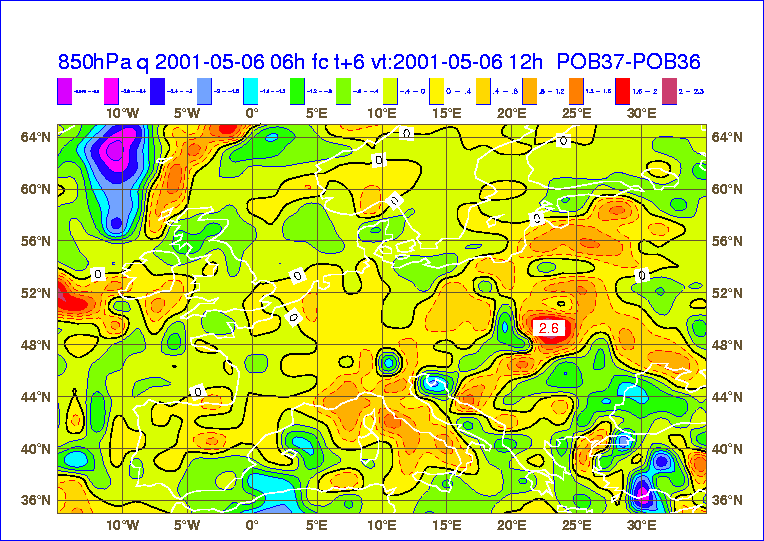
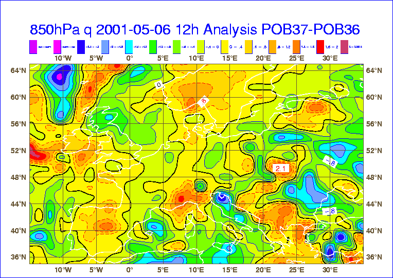
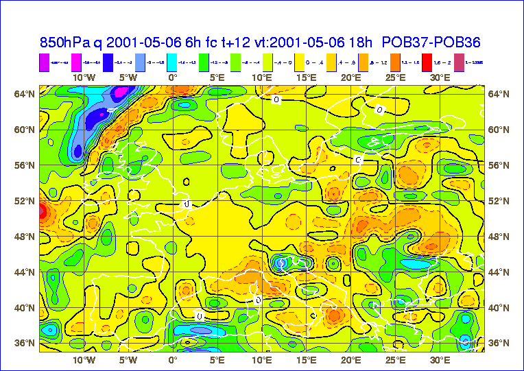
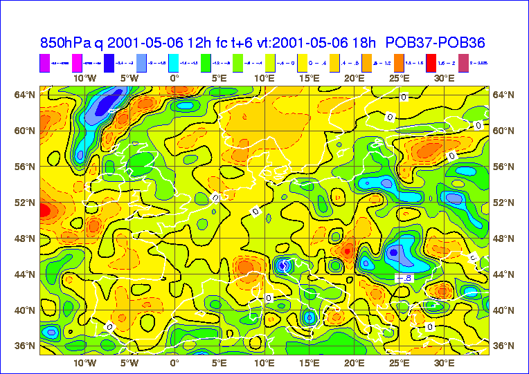
Figure 2 : Same as for figure 1, but for specific humidity (isolines of 0.4 g/kg).
Perspectives
In the near future I plan to study the geographical variability of the background and analysis errors. Moreover, I intend to compare the structures functions of the background errors estimated by the Analysis Ensemble Method and by the NMC method.
Improved representation of boundary layer
Introduction
Wind is a meteorological variable with strong spatial and temporal variability. This phenomenon has influence for everyday lifetime. Knowing its structure is desirable in many branches of industry, traffic and agriculture. Except a positive wind effect as are ecological power plants for example, it has a negative part of influence too. We are able to see a destructive forcing of this phenomenon. The results are damages on buildings, accident on the traffic, some loss in agriculture and casualties. These disasters are very frequently connected with gust winds.
The meteorological models are able to predict wind structure. It is very useful instrument, which can save a lot of people works in the dangerous events. This is one of the reasons why we want to improve a weather prediction. We do not consider a wind variable only at this moment. The gust wind has a relation with turbulent processes. We can observe eddies (irregular swirls). Their size varies from millimetres to kilometres. Nowadays the meteorological models can do a simulation of atmospheric processes with resolution about 10 m. These results can be used only for scientific study. This high resolution consumes a lot of computer time. It causes that weather forecast models can not work with this resolution. The result is that forecast models outputs are only mean variables. Horizontal resolution of the models is too small to represent correctly a turbulent motion. One can say, that some kinds of processes are beyond the model "visibility". We know that absence of this process deteriorates the weather forecast. In this reason the subgrid events implementation are done by parameterisations in the model. In the final effect it has influence on the momentum, energy and the moisture transfer.
The energy spectrum of turbulence is not homogeneous at reality. Nevertheless, we often assume that turbulence is a random process with independence on position, what is a definition of homogeneous turbulent process. Away from boundaries and from a stable stratified atmosphere this assumptions work correctly. Resolved eddies are isotropic and small energetic eddies can cascade until viscosity dissipation. In other cases anisotropy is assumed. Near the wall, the size of energetic eddies becomes proportional to the distance from this barrier. Increasing the resolution, mainly in the vertical direction, creates a problem with grid anisotropy and does not describe the situation correctly. There is a problem in representing subgrid scale processes (switch between the grid-size computation and parameterisations).
In the model ALADIN a "Flux-Gradient" approach is used for parameterisation. Turbulent fluxes are proportional to the local gradient of the mean field. The eddy coefficients are determined by factor of turbulent transfer. The crucial item for the result is a correct definition of these coefficients. Stability of air and wall distance are the main factor in this case. The mixing length, which has a dependence on wall distance and measures the average eddy size, is used for computation. The Monin-Obukhov similarity theory with empirical stability function is used. There is consideration of a surface influence by friction variables (friction velocity, potential temperature). Above the surface layer, the turbulent fluxes are computed as diffusive fluxes. The needed fluxes have been computed with this shortened description of cycle operations. Model ALADIN computes physics before the dynamics. Some mass variable demands this entry. It manifests on flux computation too. The vertical diffusion coefficients are computed at time "zero", while the split-implicit algorithm, which has origin on vertical diffusion equation, makes them act at time of "forecast". Some coefficient fibrillation problems connected with numerical scheme computation appear in stable stratified atmosphere. For this reason was developed an "anti-fibrillation scheme" (Bénard et al.), which prevents these oscillations.
The showed difficulties can be partly prevented by choosing the right variables at convenient equations in numerical model. The literature and knowledge advert, that turbulent kinetic energy (TKE) can touch problems with energy transfer and interrelation between subgrid and resolved scale. Implementation of these variables enables us to put new features and relationships among diagnostic and prognostic variables.
Summary of Activities
During the my stay in Royal Meteorological Institute of Belgium, November 2001 to March 2002, supported by ALATNET Training Network, I concentrated my work on the following scientific topics :
- Deriving equation for the unknown fluxes from perturbed part of Navier-Stokes equations.
- Constructing mean kinetic energy equation as a prognostic variable. We do an analysis of the energy transfer relationships on spectral space between energy production and dissipation terms with energy spectrum tensor. This knowledge allows us to examine this equation as a function of the wave numbers or of the eddy size.
- Solving a closure problem (1 & 1/2) with using a finite number of equations. Remaining terms we approximate with known quantities. Sommeria hypotheses were applied for statistical moments expression. Parameterized terms (statistical moments) were expressed by dependence on the turbulent kinetic energy (TKE).
This approach requires initialisation of TKE at beginning of computation. There is a problem, because TKE is a statistical moment which is characterised by subgrid properties. We investigate this problem.
Eddy length scales (viscosity length and dissipation length) are still free parameters and their expressions are needed to close our system of equations. We can see a lot of methods for determining these parameters in literature. We use a spectral characteristic for their determination.
During the whole period I study a model ALADIN, especially its 1d version. I concentrate on physics computations on this model. I try to find effective way of implementation received knowledge. I studied a literature and new articles for improving knowledge about parameterisation.
Summary of findings
Implementation of the new parameterisation schemes requires solving theoretically a lot of partial and essential problems. In other case, the implementation of these knowledge asking for good overview of model structure and interstage coupling of model physics and dynamics.
From grid construction follows that parameterized processes have different properties at horizontal direction than at vertical direction. Atmospheric turbulence has anisotropy properties, which is an essential fact from nature (effect of buoyancy force). This must be respected at SGS modelling.
From spectral analyses and literature is obvious, that the energy equation at desired form describe the inertial and the buoyancy subrange well. The TKE gives good results and it is applicable for solved problem. We work with three dimensional TKE but we are concentrating on the vertical parts of TKE only, what is applicable well in GCM (Global Circulation Model) or at mesoscale models. For economy and computer ability of computation we retain at full form equation for turbulent energy only. After application of Sommeria's hypotheses (except the turbulent energy equation), what is applied simplifications and tensor decomposition to the isotropic and anisotropy parts, we get formulas for the statistical moments. TKE remains a prognostic variable, while for other statistical moments simplifications are used. The main idea was to express the statistical moments with dependence on TKE. In this manner the properties of turbulence are directly retained for our statistical moments. The expressions contain directly turbulent kinetic energy as moderate prognostic variable. This feature allows us dispose exchange coefficients with "history" of turbulence evolution. We suppose that this proceeding can simplify a current ALADIN parameterisation and it allsow us to escape for example anti-fibrillation scheme. The stratification of the atmosphere is directly included on exchange coefficients by air stability function.
TKE equation employs virtual potential temperature. If we use virtual potential temperature as thermodynamic variable, it allows us to degrade the number of equations. However model ALADIN works with potential temperature and humidity fluxes. These fluxes can be expressed by conversion terms. Here one can discus, if we do not lose a possibility to manipulate with variance of potential temperature and humidity independently.
From our expressions the exchange coefficients have a dependence on TKE. The structure of the equation system requires initial value of TKE. We have no possibility without additional assumption to compute subgrid values in the model. The preferable algorithm is to use similar algorithms for initialisation as for next computation. Initial value is computed from TKE equation with using stationary simplification and neglecting advection terms. This expression contains a simplified function of air stability now. The original stability function has a dependence on TKE (Redelsperger number), while simplified function has dependence only on Richardson numbers. Result has desirable form for initialisation of TKE and our statistical moments.
Next task was specified eddy length parameters. Concerning a property of our equation we abandon the current ALADIN manner eddy length computation. The energy density function is expressed by convolution integral of air stratification function and energy density function in neutral stratified atmosphere now. The simplification is used for computation of eddy length parameters. We expected that air stability has a similar influence on every wave numbers. Exactly it is valid only for neutral stratification. This approach is used for computation of a length parameters only. Final result for density function is computed from convolution integral. It corrects well our simplification.
As we told above, TKE directly measures an intensity of turbulence and it can afford new knowledge for parameterisation. It is clear, that adding this equation as prognostic equation has positive effect for properties of parameterisation, although it increases a number of unknowns.
Further enhancement can be done by non-local view of parameterisation. Non-local approach uses not only adjacent region for parameterisation. It can take into account the effects of all various sizes eddy from far location.
Current works
Concerning the wide spectrum of problems, which are solved, I study the literature continuously. Now we are concentrating on stability of nonlinear prognostic TKE equation. We start to implement reached results to 1d model. We implement new exchange coefficients for needed fluxes and statistical moments. It is connected with initialisation of TKE. Tuning an integration constant will be necessary.
I shall take part in the ALATNET Seminar on Numerical Methods in Slovenia at the end of May 2002. In June 2002 I shall attend a workshop on the 12th ALADIN Workshop on Scientific Development and Operational Exploitation of ALADIN model.
Reformulation of the physics-dynamics interface for the non-hydrostatic model.
The research evolved into various smaller topics which have been studied during the first part of my stay in the IRM in Brussels :
1. As a continuation of my PhD work in Météo-France I studied the properties of the predictor-corrector time integration numerical scheme for the hydrostatic 3d model compared to the properties of the uniform acceleration semi-Lagrangian trajectory scheme applied to the 3d model. The work was concentrated around implementing the uniform acceleration trajectory scheme into a more recent cycle of the ARPEGE/ALADIN weather forecasting system. The idea is to compare the quality and the efficiency of the two methods for the 3d model. It was demonstrated with a simplified 1d model that the advantage of the predictor-corrector method dominated the uniform acceleration trajectory scheme only slightly in terms of quality while it was considerably more expensive. However, the conclusion for the real 3d model cannot be taken only on the basis of the experiments with the simplified one. The last motivated this comparative study. The preliminary results show domination of the predictor-corrector method against the uniform acceleration semi-Lagrangian scheme applied to the hydrostatic 3d model. The reason that the advantages of the predictor-corrector scheme compared to the uniform acceleration trajectory scheme are more important in the 3d model than in the simplified 1d shallow-water one can be explained with the fundamental difference between the two models. This is the vertical dimension in the 3d model and its complexity in case of a hydrostatic dynamics. The problem is that the vertical motion is not a degree of freedom in a hydrostatic atmospheric model. It is limited by the hydrostatic assumption and the governing vertical momentum equation is reduced to a diagnostic hydrostatic relationship. The vertical velocity and therefore the vertical acceleration are diagnostically derived from the continuity equation. The derivation of the vertical acceleration involves also the rest of the model dynamics. Thus, the vertical acceleration for a hydrostatic model is only an anticipative estimate of how the model should evolve along the next time step. However, on the horizontal there is an explicit acceleration defined by the horizontal momentum equation. The simplified 1d model is representative mostly for this part of the 3d model dynamics. The predictor-corrector method has the advantage to incorporate the entire model dynamics in the construction of the numerical scheme for the vertical semi-Lagrangian trajectory. Thus, it takes into account the entire spectrum of procedures designed to satisfy both the numerical and dynamical constrains imposed to the representation of the vertical motion in the hydrostatic 3d model ARPEGE/ALADIN. That is a possible explanation of the pronounced domination of the predictor-corrector method on the uniform acceleration trajectory scheme in the 3d hydrostatic atmospheric model ARPEGE/ALADIN.
2. There is a forthcoming need of some of the Aladin partners to implement a very high resolution version of the mesoscale model by using its current state of scientific development. This inspired the second study on dynamics which occupied my time during the firs part of my stay in Brussels. The most rapid way to test the feasibility of this idea with the Aladin model was to test first a similar procedure with the simplified 1d shallow-water model. There is a limited-area version of the simplified 1d "shallow water" model developed by Piet Termonia at IRM, Brussels. It was used to test the response of the model to a very big difference between the resolution of the parent 'global' model (though simplified 1d one) and the limited-area model. The most important and probably the only possible significant difference between the two models in terms of forcing was the resolution of the orography. The preliminary results are not favourable to such a drastic jump in resolution going from the parent model to the limited-area one. Despite our effort to smooth out the transition, the behaviour of the very high resolution limited-area model was discouraging. The idea that is being tested currently is the so-called method of telescoping or, in other words, increasing gradually the resolution until reaching the desirable one. This is most probably going to show acceptable results. However, it is an expensive solution.
3. The research on the problem of the interface between physics and dynamics is divided into two parts. The first part which has already been undertaken concerns theoretical study of the problem, reading literature and defining the current state of the problem in both hydrostatic and non-hydrostatic version of Aladin. There are a number of techniques that can be used for combining the dynamics and physics contributions. It is linked to the semi-implicit feature of the model. The different techniques are to be re-examined for both hydrostatic and non-hydrostatic version of Aladin. Eventually a new strategy for the case of non-hydrostatic dynamics may be designed and explored.
4. Other activities :
In June 2001 I participated the ALATNET seminar on data assimilation in Gourdon, France.
In July 2001 I registered to attend the SRNWP mini-workshop on numerical techniques in Bratislava, Slovakia. However, I could not attend due to administrative problems.
In October 2001 I presented my research activities and plans on an internal seminar at IRM.
In 2001 while in Brussels I also worked on the revised version of our publication: A refined semi-Lagrangian vertical trajectory scheme applied to a hydrostatic atmospheric model, by I. Gospodinov, V. Spiridonov, P. Bénard and J.-F. Geleyn, 2002, Quart. J. Roy. Meteor. Soc. , 128, 323-336.
In May 2002 I will attend the ALATNET seminar on numerical methods in Slovenia and in June 2002 I will attend the 12th ALADIN workshop on operational and scientific developments in ALADIN in Medulin, Croatia.
Extensive study of the coupling problem for a high resolution limited area model
Limited area models need information about the state of the atmosphere outside the integration area, so one of the inherent problems is the specification of the lateral boundary conditions. A number of studies have demonstrated that LBCs of LAMs can have a significant impact on the evolution of the predicted fields through the propagation of boundary errors onto the interior of the domain. As each prognostic variable is prescribed at each lateral boundary point the result is over-determination (ill-posedness) and a consequence is partial reflections that propagate these errors back in the integration area. In order to introduce lateral boundary information coming from large scale model and to damp the reflection produced by limited area model, the Davies-Kallberg relaxation scheme (Davies 1976) is used in ALADIN. This method accepts its ill-posedness and tries to damp reflected spurious waves by using a relaxation zone. Coupling means that every time step the values of the ALADIN model, obtained without any influence of the coupling model, are combined with the values interpolated on the ALADIN grid starting from the coupling model. During this first ALATNET stay the study has been concentrated on the study of the presently used relaxation scheme and on the improving of a new method for coupling. The investigation of weaknesses of the Davies-Kallberg scheme and possible enhancement of it was the first step. This was tested with 3d numerical experiments on Christmas storm from December 1999. In this case two deep cyclones developed in the middle Atlantic and passed quickly through Western Europe. Some integrations of standard ALADIN model, using hourly ARPEGE global model forecasts as coupling files and applying them as lateral boundary conditions for the LACE domain, were done. The purpose was to study the impact of coupling frequency by comparing the depth of the cyclone in the coupling and coupled model near the time of entering domain using MSLP post-processed fields and observing the entry time in the domain. 25.12.1999 Christmas storm case Starting from the given data the model arrives to a surprising solution with 6 hours coupling frequency of updating the boundary files. For 18 hours forecast valid for 06UTC in 26.12.99 the cyclone is missing (Fig1a), meanwhile for 3 hours coupling frequency, the pressure field has the value 976 hPa (see Fig1b) and with hourly coupling frequency the same hour, the cyclone has the deepest value 974 hPa (Fig1c) and the closest to the forecasted field by ARPEGE (Fig1d), the reasonably good for that day. 27.12.1999 Christmas storm case Using 6 hours coupling frequency in integration for 2 h with coupling files from global model the plotted MSLP field has 984 hPa value for the second cyclone at 21 h UTC for 27.12.99, for the same hour a value of 982 hPa using 3 hours coupling files frequency in integration of the model and the deepest value again was obtained using hourly coupling frequency 980 hPa, as in the case of the first storm. For the coupling field obtained directly from global model there is a minimum value 977 hPa from all of them. As we expected the closest value to reality in both cases was that one obtained through hourly frequency of coupling. Discussion : because the system was moving very fast it happened that it didn't appear in the coupling zone of the model at the coupling times. ALADIN has no chance to forecast the storm if the cyclone genesis process is outside its domain, as it gets any information through lateral boundary conditions on the existence of such a system. Even if the coupling model forecasts the system, the coupling scheme can fail to pass the information to the LAM, and this was the case. In addition, the forcing field is not the forecasted field of the coupling model for the given time, but the field obtained by temporal interpolation of two forecasts of the global models. If the system had no trace on the coupling zone (first time is outside the domain, next time is fully entered inside the domain), it cannot be forecasted by LAM. This can happen because the coupling model passes the information to the LAM only by its fields over the coupling zone at discrete times. Next step is introduction and testing of spectral coupling, considered to be a solution for the problems described above, offered by the fact that ALADIN is a spectral model using Fourier expansions in both horizontal directions. Spectral coupling means blending of large scale spectral state vector with the state vector of the coupled model so that the blended state vector is equal to the large scale one for small wavenumbers and equal to the coupled one for large wavenumbers with a smooth transition in between. A spectral coupling scheme is built on the same analogy of the Davies relaxation scheme as an additional coupling step.
New coupling scheme provides scale selection where large scales are dominated by the spectra of the coupling model and only small scales resolved by the forcing model are dominated by LAM. The potential advantage of spectral coupling is that scales resolved by the coupled model are forced to LAM, even if the location of the system of the given scale is inside the domain. Spectral coupling cannot eliminate spurious inward propagation through the lateral boundaries, without the damping by the standard Davies scheme all waves that exit on one side of the domain would freely enter on the opposite side, but using simultaneous Davies scheme and spectral coupling the advantages of both methods are combined. This point required code development, which is going at the present moment. It looks reasonable to introduce this step after finishing semi-implicit scheme in spectral space but before applying horizontal diffusion. In principle the idea is to read the spectral coupling fields, introduction of a large scale buffer, make the time interpolation and blend ALADIN spectral fields with interpolated large scale ones by the use of the spectral alpha weight function. From technical point of view in the present the new spectral coupling scheme is working without major problems. The tests were done assuming mono-processor running of the operational model on Slovenia domain. Some figures with representaTION OF MEAN SEA LEVEL PRESSURE field are showed below. In Fig2 we have the result of integration of model using only classic gridpoints coupling scheme and in the next one (Fig3) we can see the result of the model using the spectral coupling scheme. Now the tuning of spectral alpha is absolutely important for the next step as well as the code version for multi-processors for optimal computation time. In order to avoid too strong external forcing we consider the retuning of alpha function of gridpoint coupling and also we keep open the possibility not to apply the spectral coupling at every time step of integration of the model by introduction of a step frequency.
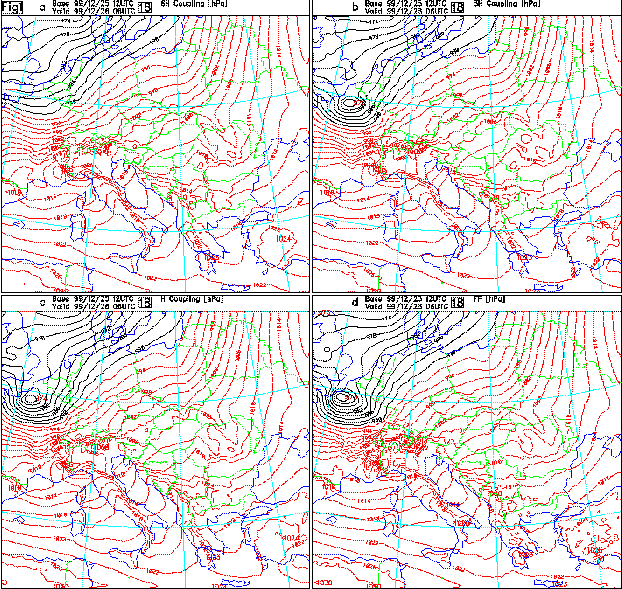
Figure 1 : Impact of coupling frequency on mean-sea-level pressure field forecasted for 10 hours valid for 26.12.99 06 h UTC. a) MSLP field of ALADIN using 6 hours coupling files. b) MSLP field of ALADIN using 3 hours coupling files. c) MSLP field of ALADIN using 1 hours coupling files. d) MSLP field of ARPEGE forecast.
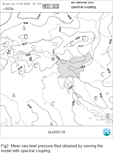
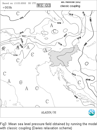
References :
Davies, 1976 : "A lateral boundary formulation for multi-level prediction models", Quart. J. Roy. Meteor. Soc., 102, 405-418
A. Mc Donald, 1997 : "Lateral boundary conditions for operational regional forecast models" a review. HIRLAM technical note n° 32
R. Lehmann, 1993 : "On the choice of relaxation coefficients for Davies lateral boundary scheme for regional weather prediction models", Meteorology and Atmospheric Physics, 52 , 1-14
Gabor Radnoti, 2001 : "An improved method to incorporate lateral boundary conditions in a spectral limited area model"
M. Janiskova, 1994 : "Study of the coupling problem". ALADIN note
Study of the relationship between
turbulent fluxes in deeply stable PBL situations and cyclogenetic activity
Introduction
The situations with rapid cyclogenesis in northern Atlantic, that appeared in December 1998 and 1999, increased the effort to understand and to predict such severe events.
The recent research on relationship between physical parametrisation and predictability of cyclogenesis has shown, that the way of describing the turbulent transport has significant influence on the model results. More surprising fact is, that considerable model sensitivity on vertical diffusion we can find in areas with high static stability in the planetary boundary layer (PBL). These areas were probably crucial for the real development of the December 1998 storm and for it's prediction. This knowledge led to adjustments in the vertical diffusion scheme, including the shape of the mixing length profile and limitation of Richardson number in very stable cases. The aim of the current scheme in the ARPEGE and ALADIN model and of it's future development is to describe better the cyclogenetic activity and to be not worse in other outputs of the model computation (e.g. by forecasting inversion or convection). This requires more realistic approach in modeling of the turbulent transport, thus forcing us to study in more details the interaction between the PBL processes and cyclogenesis.
Summary of activities
Theoretical study of the present parametrisation scheme in the ARPEGE/ALADIN model, including the vertical profiles of mixing length, Richardson flux number and computation of exchange coefficients for momentum and heat. The purpose of this study was to understand the sensitivity of the scheme using different setup of parameters and varying the Richardson number.
Study of the 1998 storm evolution, using model analysis and forecasts of several parameters (e.g. mean sea level pressure, geopotential, horizontal wind speed and direction, potential temperature, potential vorticity, vertical velocity etc.) and vertical cross sections in the areas of interest. The diagnostic fields of 1.5 PVU (Potential Vorticity Unit) height were compared with METEOSAT satellite images in water vapour and infrared channel.
Experimental runs with different setup of parameters of vertical turbulent transport, mainly changing the Richardson number limitation for heat exchange. The range of the forecasts varied from 36 to 96 hours (but with equal validity), thus studying not only the dependence of the results on different initial conditions but in the same time looking for the period of biggest influence of vertical diffusion parameterisation.
Experimental runs with adjustments of shallow convection scheme in the Richardson number computation. Looking for the areas of highest sensitivity on vertical diffusion via comparing the results with good and wrong predictability of the storm during the period of impact.
Visualisation of vertical profiles (cross sections) of potential temperature, wind, Richardson number and turbulent fluxes of momentum and heat in above mentioned areas to understand the relationship between the local conditions and the impact on the life cycle of the predicted cyclone.
Preliminary results
The first results with the currently used scheme of vertical diffusion in the model showed similar influence of Richardson number limitation on cyclogenetic activity like was observed during earlier experiments done in this topic. It seems, that increasing the rate of heat exchange in stable PBL allows us to forecast rapidly developing cyclones, as it was in the case from December 1998. Nevertheless, it comes from more detailed analysis (using vertical cross sections of various parameters or the 1.5 PVU height), that by overlapping certain threshold, the structure of the cyclone is missed, though we have almost perfect forecast of mean sea level pressure (Fig.1-4).
Introducing the adjusted, time-averaged parameter of shallow convection gave apparently better results in the case of December 1998. This knowledge is useful, because it allows to forecast deeper cyclones without too big increase of the heat exchange, thus avoiding the problem of inversion erosion.
Forecasts, which started from different initial conditions, show , that the scheme has significant impact during the very early stage of the observed cyclone, far before it has rapidly deepened near British Isles. This explains, why the forecasts for shorter time period (36 to 72 hours) were less successful, as the forecasts on 84 or 96 hours and it helps us to find the most problematic areas.
Finally, the comparisons between the two runs with good and bad predictability of the storm depicted the regions, which were probably the most important for further evolution of the cyclone. These could be found southerly from Iceland and in the area of Newfoundland and Labrador. Outputs of various pressure levels fulfilled our former expectations, that the biggest impact of vertical diffusion is related to the levels beneath or at the top of the PBL. The vertical cross sections give the evidence of relatively high static stability and locally increased values of Richardson number.
Conclusion and future plans
The importance of the low atmospheric levels in predicting cyclogenesis was already shown by Rabier et al. (1993). During the FASTEX experiments in 1997 a lot of investigations were done to understand the processes of cyclogenesis in Northern Atlantic, touching also the influence of diabatic heating (Mallet et al ., 1999). Relationship between the stable PBL layers and cyclogenesis seems to be a less known problem, which is still present using the current scheme of vertical diffusion. The research should continue with tests on more situations (e.g. the storms of December 1999 and cyclonic situations during the 2000/2001 seasons). Further improvements can be done by choosing another representation of the mixing length profile or by more realistic description of PBL height in the vertical diffusion parameterisation.
References
Rabier F., Courtier P., Herveou M., Strauss B., Persson A., 1993, Sensitivity of forecast error to initial conditions using the adjoint model. ECMWF Technical Memorandum n° 197, 29 pp.
Mallet I., Cammas J.-P., Mascart P. and Bechtold P., 1999, Effects of cloud diabatic heating on the early experiment of the FASTEX IOP17 cyclone, Quart. J. Roy. Meteor. Soc., 125, 3439 - 3467
Figures:
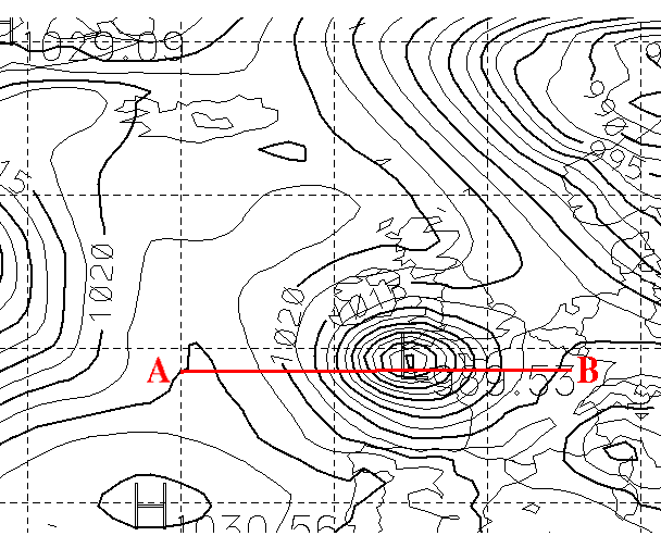
Figure 1 : 96 hour forecast of mean sea level pressure valid to 00 h UTC, 20 December 1998. The red line denotes the position of the cross sections starting from the initial point A leading to point B (see Fig. 2-4). The forecast was done with decreasing of the parameter USURID in the vertical diffusion scheme from the current reference value 0.035 to 0.015. In other words that means stronger decrease of Richardson number limitation with height with the consequence of increasing the turbulent exchange of heat around the top of the PBL, mainly in regions of strong stability. The forecasted pressure in the centre of the low was almost the same as it was estimated from the observations (nearly 990 hPa).
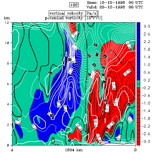
Figure 2 : 96 hour forecast of vertical velocity field (coloured and black isolines) superimposed with the field of potential vorticity (white contours) valid to 00 h UTC, 20 December 1998, using the value of USURID=0.015 as in Fig.1. The profiles of the upper air fields are quite different comparing to the model analysis in Fig.4.
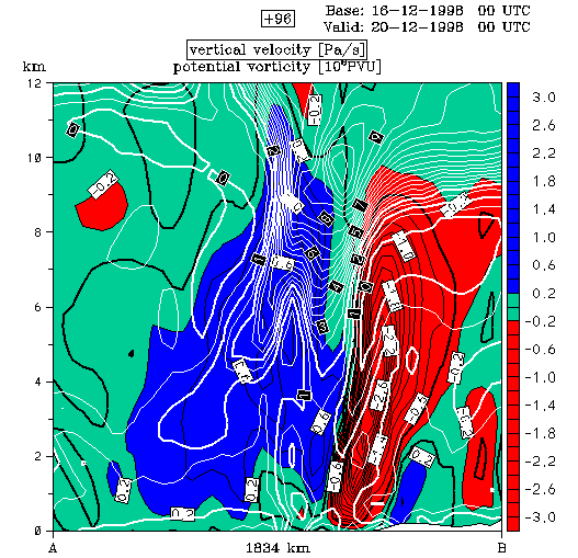
Figure 3 : 96 hour forecast of vertical velocity field (coloured and black isolines) superimposed with the field of potential vorticity (white contours) valid to 00 h UTC, 20 December 1998. Forecast was done with increasing of the USURID parameter from the reference value (0.035) to 0.055. Decreasing of heat exchange in the stable PBL gives results with less deep cyclone but with profiles of potential vorticity or vertical velocity closer to the model analysis. Direction of the cross section is in Fig.1
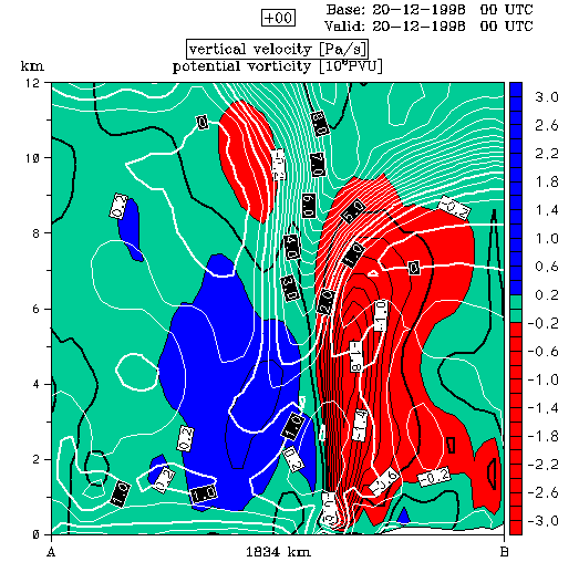
Figure 4 : Model analysis of the field of vertical velocity (coloured and black isolines) superimposed with the field of potential vorticity (white contours) in vertical cross section marked in Fig.1.a). Valid to 00 h UTC, 20 December 1998.
Research Work
During this year I have continued to investigate problems associated with the lower boundary condition, in the non-hydrostatic formulation of ALADIN. The principal research tool for this work is the two-dimensional vertical slice model, used to compute idealised flows over mountains. My early work on this led to an improvement in the estimation of three-dimensional divergence. This led to significant improvement in the accuracy of the model results. However, this improvement was obtained only when the mountain height was relatively small, or if the Eulerian time scheme was used. These are unacceptable limitations, if non-hydrostatic ALADIN is to be an operational forecast tool. The model should be able to handle complex mountainous terrain of realistic height, while also employing the semi-Lagrangian time scheme, which offers stable simulations with a longer time-step than the Eulerian scheme.
The methodology applied to the estimation of divergence may also be applied to other terms in the non-hydrostatic equations of ALADIN. These terms relate to the computation of the pressure gradient force in the horizontal and vertical momentum equations. Modification of these terms did not result in any further significant improvement.
A long sequence of tests eventually led to the following conclusion. In non-hydrostatic ALADIN the vertical gradient of vertical wind (referred to as vertical divergence) is used as a prognostic variable. There are various ways in which this variable may be defined, depending on how vertical differences in geopotential are measured. For instance, we may use the semi-implicit reference profile to calculate these differences, or the true geopotential of the simulated atmosphere. Various hybrid combinations are also possible. All of these variables lead to a system of discretised equations suffering the same basic problem in the specification of a lower boundary condition. We wish to impose a free-slip condition at the lower boundary. This is a constraint relating, through the gradient of the orography, the horizontal and vertical components of wind on the lower boundary. If this boundary condition is to be expressed in terms of vertical divergence, then extra assumptions must be introduced about the nature of the flow just above the lower boundary. The way in which vertical divergence should be adjusted in order to meet such a boundary condition appears to be entirely arbitrary. At least we can say, that no satisfactory method has so far been found.
One solution, therefore, is to use vertical wind as a prognostic variable, in place of vertical divergence. This allows the free-slip lower boundary condition to be introduced in its most natural form, without the need for any extra assumptions. The result of this change is shown in Figure 1 and Figure 2. Figure 1 shows the vertical velocity for a potential flow test. The solution should be steady, evanescent (no propagating waves) and anti-symmetric about the axis of the mountain. On the left is the result obtained using vertical divergence as prognostic variable; on the right vertical velocity has been used as prognostic variable. Figure 2 also shows vertical velocity, this time for a stably stratified, nonlinear, non-hydrostatic flow test. The solution should be steady and contain a gravity wave response with strong downstream propagation. On the left is the result obtained using vertical divergence as prognostic variable and, on the right, that obtained using vertical wind prognostically. In both cases, due to the lack of an effective lower boundary condition, the first scheme suffers a severe defect directly over the mountain.
Future Work
Although the use of vertical wind as a prognostic variable allows for a better formulation of the lower boundary condition, the resulting scheme still does not allow the full potential of the semi-Lagrangian (SL) scheme. At the large time-steps allowed by the SL scheme additional spurious behaviour occurs in both the idealised tests presented above, even when vertical wind is used prognostically. This is probably connected with the well-documented phenomenon of ``orographic resonance'' observed in SL schemes. One standard remedy is to use temporal decentering and this does provide some improvement to the results in this case. My investigations will, therefore, continue in this direction, while also examining other aspects of the SL scheme likely to be implicated. For instance, at large time-steps problems arise connected with the calculation of fluid parcel trajectories. Unless the orography is sufficiently well-resolved, these can be liable to significant error when terrain-conforming coordinates are used.
Other Activities
During 2001 I attended the following meetings.
June
ALATNET Seminar on Data Assimilation in Gourdon, France. The course provided a broad overview of all aspects of the subject, from the theoretical basis to practical details about quality control of observational data. Selected topics were also examined in great detail.
July
SRNWP Workshop on Numerical Techniques in Bratislava, Slovakia. This workshop brought together specialists from several European countries. Presentations and discussions examined various issues of importance to short-range numerical weather prediction.
October
EWGLAM/SRNWP Meeting in Cracow, Poland. This meeting brought together representatives from all the European groups involved in limited area numerical weather prediction. The meeting included discussions about cooperative activities between the member groups, in addition to scientific presentations.
Future Training
In May 2002 I shall attend the ALATNET Seminar on Numerical Methods for Meteorology, to be held in Slovenia.
Figure 1 : Potential flow test. Prognostic variable is vertical divergence (left), vertical velocity (right).
Figure 2 : Nonlinear non-hydrostatic flow test. Prognostic variable is vertical divergence (left), vertical velocity (right).
Sensitivity studies using a limited-area model and its adjoint for the mesoscale range
1. Introduction
The development of the adjoint model is primarily oriented through data assimilation and predictability applications. However, since it is able to relate the origin of a numerical forecast failure to the errors in the initial data it has been used for sensitivity experiments. The latter approach was proven to be successful especially when a global or a low resolution regional model was taken as a tool for studying rapid evolving cyclogenesis. One of the reasons is that the adjoint model is able to represent with a reasonable accuracy phenomena linked to baroclinic instability. Thus, even an adiabatic adjoint model or one including a very simple parameterization of the surface wave drag and vertical diffusion can be useful. For a limited- area model currently utilized for short range weather prediction, the moist processes which are strongly nonlinear start playing a crucial role. This creates additional problems for a linear model and hence the need of improving the physical description of the atmospheric processes in the adjoint model. Despite of difficulties, the adjoint technique remains a powerful candidate for high frequency data assimilation into a limited-area model.
2. Objectives
The main goals of this work may be summarized as follows:
- the usage and evaluation of the adjoint of a high resolution limited-area model;
- the computation of the gradients of a forecast error cost function with respect to the initial conditions using an adjoint model with different linearized physics;
- the study of the initial model errors which lead to a forecast failure.
3. Methods and tools
The model considered in our studies was the high resolution, spectral limited-area model ALADIN with 31 vertical levels and a grid size of 9.5 km. A triple nested model with the same number of vertical levels and 8 km grid size was also used. Sensitivities were computed at full model resolution. Both nonlinear and adjoint versions have been run using an Eulerian, leapfrog, advection scheme with 60 s time-step. The integrations for the gradient computations were carried out over a 6 h period. The misfit between the model solution and the analysis available at the verification time was quantified by a forecast error cost function. Forecast error is defined as a difference between the nonlinear forecast and a verifying analysis taken as the truth of the atmospheric state. The squared norms utilized were the so-called dry and moist total energy. The norm is called dry when there is no term in it involving specific humidity. The adjoint of the tangent linear ALADIN model was used for providing an estimate of the gradients of the forecast error cost function with respect to the initial conditions. It includes a package of simplified and regularized physical parameterizations for computation of radiative fluxes, vertical diffusion, subgrid scale orographic effects, large scale precipitation and deep convective fluxes. The regularization consists in removing some thresholds in the physical parameterizations that can affect the range of validity of the linear approximation. Since this package was developed with the aim of using it in the incremental four-dimensional data assimilation carried out within a global spectral model, an assessment for limited-area high resolution model was needed.
4. Summary of results
Several sensitivity experiments using the simplified physical parameterization schemes for the gradient computations have been carried out. The package is a modular one, i.e. it is possible to activate at once one, two or all schemes together. This is an important feature because it allows us to assess a particular physical parameterization scheme which can be responsible for deficiencies in the linear model performance. The results obtained during our experiments, might be divided into two main groups: on the one hand the gradient pattern and magnitude, and on the other hand the sensitivity forecast run. It was seen that an adjoint model including a sophisticated description of the physical processes is very sensitive to the trajectory. This is especially stressed when for the gradient computation the moist schemes such as large scale precipitation and deep convection were used . The linearized and regularized large scale precipitation scheme triggered strong instability in the adjoint model. This problem was cured by retuning the coefficients for shape and shift of the regularization function. The adjoint model is able to retrieve the sensitive area in the initial conditions. This area tells us where one should have a look for the errors which may affect the forecast.
Starting from modified initial conditions, sensitivity integrations on selected cases have been performed in order to improve the 6 hour precipitation forecast. Comparing the sensitivity and the control forecasts, the results have revealed to be case dependent. For some cases, the impact was rather neutral. For others, the precipitation forecast was improved, although the degree of the improvement was primarily a function of the amplitude of the initial perturbation. Furthermore, it was demonstrated that the verifying analysis does not play an important role as a true state of the atmosphere. Indeed, if the analysis file is replaced by a previous forecast file valid for the verifying time, the sensitive area remains the same, although the magnitude and the pattern of the gradients change. A forecast started from initial conditions modified with a perturbation of a realistic and large enough amplitude introduced in this area will evolve in the desired direction. This may lead to the conclusion that the forecast can be improved even if the failure is dominated by a growing non- linear error structure in the initial data, leading eventually to the triggering of a convection event. For the results with neutral impact, the misforecast is presumably not only a matter of initial data but more specifically of lateral boundary conditions.
Systematic qualitative evaluation of the high-resolution non-hydrostatic ALADIN model
The second part of the first stay at the research-centre in Ljubljana was used for testing, whether currently used settings in physics and dynamics for the ALADIN-model are suitable for very high resolution (approx. 2.5 km) and beyond and if the expected advantages of using non-hydrostatic dynamics already appear on this resolution.
One case, which was chosen to try to answer this questions is the 20.9.1999, which is part of one MAP-I(ntensive) O(bservation) (P)eriod. The forecasting domain includes part of north-east Italy, western Slovenia and parts of north-west Croatia. Domain size is 80*80 points (without E-zone) and the main synoptic feature is a front. It approached from the west, had its main activity in northern Italy and was already weaker when affecting the target-domain, but still causing significant amounts of rain.
1. Generalities
It has to be expected that forecasted vertical velocity and precipitation fields are strongly influenced by the mountains located in the northern part of the domain and at the Croatian coast as well. Several experiment runs with different settings were made which led to the following basic conclusions:
A: Down to 5 km resolution the currently used settings can be used without any problems and forecasted fields look reasonable.
B: Increasing the resolution down to 2.5 km leads to wavy precipitation fields over the sea and to unrealistically strong precipitation minima and maxima, following the model orography, if the 'original' model orography is used
C: The differences between using non-hydrostatic or hydrostatic dynamics are small compared to other changes in the settings. (This is valid for both 2.5 km and 5 km resolution.)
2. Details
Concerning B: (see Figure 1) it shows the 2 hour forecast of the 2 hour-precipitation field on 2.5 km resolution The unrealistic precipitation pattern over the sea can easily be recognized. Further one can see too many and too extreme structures in the precipitation field over the mountainous area in the northern part of the domain, including unrealistic dry areas. To identify and cure this problem a lot of experiments have been carried out and finally it can be stated that the use of a minimisation algorithm applied on the orography is able to reduce the wavy patterns, but is not sufficient to solve the problems with the upslope maxima. This can more or less be reached, if the representation of the orography is smoother than those of the other fields, which means that orography is used on quadratic grid, while the other fields are computed on a linear grid. See figure 3 - forecast with using linear grid and coarser resolution of orography. Finally one gets the impression that with generally using linear grid and additionally using optimized orography on quadratic grid forecasted fields look most realistic. Still, some problems in the mountainous areas remain. This could be related to the missing advection of liquid cloud water and/or to the parameterisations of mountain-flow interaction in the model.
Concerning C: see Figures 2 and 4 - which show the difference fields for T850 forecast between hydrostatic and non-hydrostatic run (Figure 4) and between different resolutions of the coupling domains for two non-hydrostatic runs (Figure 2). The different coupling resolutions for the 2.5 km forecast were approx. 11 km and approx. 5 km. It can be seen that the differences for the different coupling resolutions are much bigger than those for the other case.
3. Conclusions
The main problems which appear when running the model on 2.5 km resolution are more related to the dynamical part than to the physical one. The use of linear grid, spectrally fitted, and coarser (which gives more realistic fields in the mountain regions) orography provides a basis for running the model also on very high resolution achieving acceptable results, which can serve as a basis for a systematic evaluation.
Figures
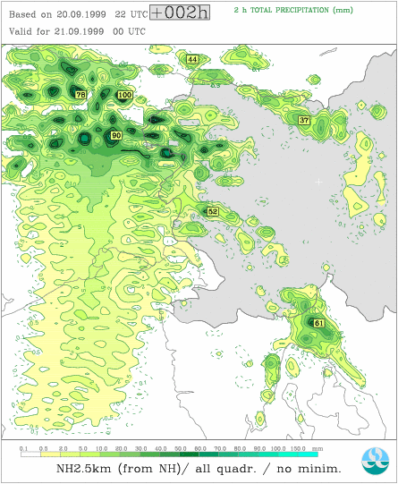
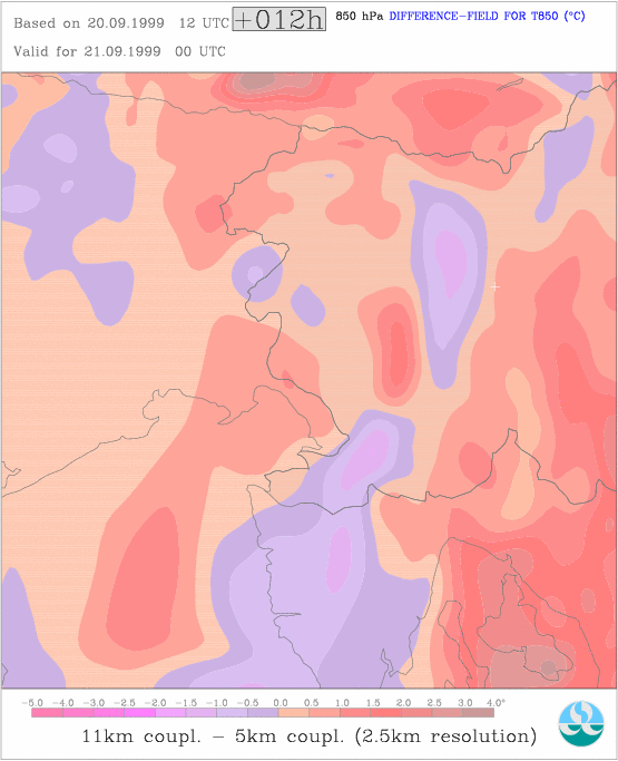
Figure 1 : NH-model on 2.5 km, all on quadratic grid Figure 2 : different coupling resolutions
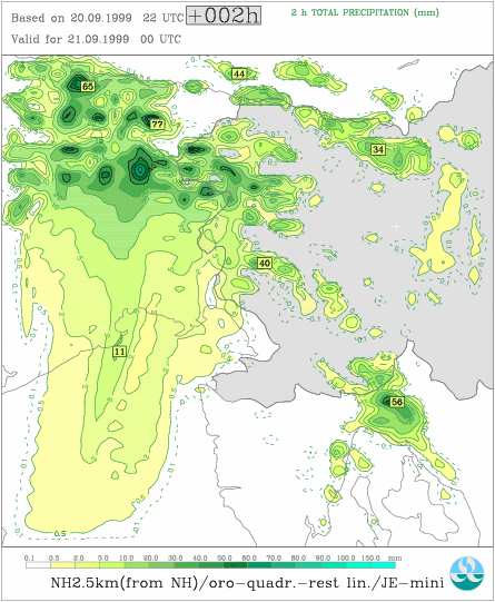
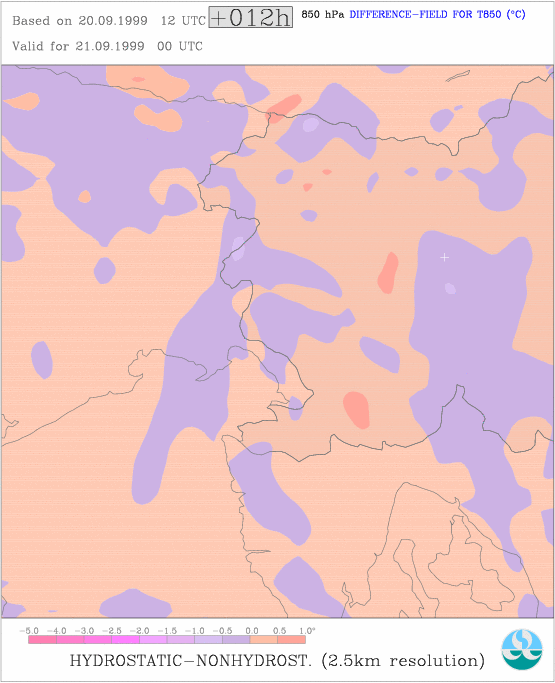
Figure 3 : NH-model on linear grid, Figure 4 : different dynamics
"minimized" orography on quadratic grid
Use of IASI/AIRS observations over land
I. Introduction
This is the study of use of observations over land from advanced infrared sounders (with spectral resolution < 0.5 cm-1) such as IASI or AIRS. Previous works were focused mainly to the data over sea. Over land the problem is the simultaneous retrieval of atmospheric profiles and surface characteristics (land surface temperature LST and surface spectral emissivity SSE). Two basic ways of such retrieval can be distinguished and the main component for both consist of the usage of ancillary information which specifies SSE behaviour or constitutes some a priori constrains. A first estimate of surface temperature can be taken from model forecast, and emissivity can be provided by climatological values depending on the land cover type.
The first part of the study comprised the inclusion of emissivity fields for chosen spectral ranges into ARPEGE climatological files. The further study will use one-dimensional framework to test the retrieval of both profiles and surface values. Then, it will be extended to three-dimensional analysis scheme.
IASI, an Infrared Atmospheric Sounding Interferometer is jointly developed by EUMETSAT and CNES an will be operational instrument on the EPS-Metop series of satellites (first launch about 2005). The IASI instrument supplies the spectra of the atmosphere in the IR band, with 8461 channels in each spectrum. This gives us great advantage of treating emissivity spectra as separated into wavebands. AIRS, the Atmospheric Infrared Sounder - to be launched in this year, will give the opportunity to test the methods developed for IASI.
2. Emissivity and Climatology
Until now in ARPEGE model, surface characteristics were just two fields - the albedo of bare soil and emissivity, but without annual changes. The emissivity (mean value over the entire spectrum) was interpolated or calculated over the final grid as a function of surface type and the maximum fraction of vegetation. The mean values of emissivity were derived from old Navy data. Such treatment of emissivity was not sufficient for our studies, so the work on the creation of new climatological fields of SSE had been started. At the beginning we divided IASI IR range into 12 equal wavebands : from 600 cm -1 to 3000 cm-1 with step 200 cm-1 . According to them, climatological fields of surface spectral emissivity were created. Two approaches of creating climatological files of SSE were used, namely with and without interpolation of emissivity. The first one was based on the global emissivity maps with the resolution of 0.5 °; over the whole world, and were created on the basis of MODIS spectral library and also 0.5 °; resolution global vegetation maps. Then, those SSE maps were taken as an input for configuration 923 (modified one) in which emissivity was interpolated to the final model grid. The second way was to assign spectral emissivity values, calculated from MODIS and ASTER data, to each model grid point with respect to surface type, percentage of land and maximum fraction of vegetation. The differences between climatological emissivity fields created on both ways were found just over land covered by vegetation. They were caused by different vegetation maps usage. To be consistent with the model vegetation cover and because of the emissivity maps were without estimation errors we have decided to use the second way of climatological files creation. The result of this work were 12 new climatological fields of SSE, figure below shows the climatological map of spectral emissivity for January and waveband 1800-2000 cm-1.
The our newest studies of the IASI transmittances in each channel shows that separation of spectra into equal wavebands are not the best to our purposes. New way of spectra separation is according to the value of transmittancy (low, medium and high) and emissivity spectra behaviour. There are 12 final bands, in lower wavenumbers they are similar to Fu-Liou bands.
Main sources of infrared emissivity were MODIS and ASTER spectral libraries, which contain respectively emissivities and reflectances of many kinds of materials. It was very important to obtain as many samples as possible for each type of land cover to calculate the emissivity background error covariance matrix. The final sample sizes are : sea water - 5 sub-samples, ice/snow - 9 sub-samples, 128 sub-samples of different kinds of soils and sands, 24 sub-samples of high vegetation (trees) and 5 sub-samples of low vegetation.
3. Background error covariance matrix - starting point
During the climatological experiments one more problem had raised, to use directly SSE or convert it to -log(1-SSE) ? The emissivity values in general are very close to 1, and they are always lower than 1, so such a change would help for the further studies with LST and SSE inversions. We checked the distribution of the errors (SSE-av(SSE)) around 0 for both kinds of data. It was done for all wavebands together and separately for each surface cover type. Results showed that it is difficult to judge the distribution of the errors almost for all surface types (except soil) because of too small number of samples, but the soil case showed that more Gaussian distribution is for the -log(1-SSE) than for direct SSE values. Afterwards for verifying if it is in general true for all data together a global sample for all types of the surface cover was prepared. The compilation of those emissivities was based on weights - measuring the importance of each surface type in the global aspect. The basis for it was taken from the ARPEGE model. In it, each surface type covers following the percentage of the globe: sea water - 53.4 %, ice/snow - 1.4 %, high vegetation - 13.5 %, low vegetation - 29.2 % and bare soil - 2.5 %. The results shows the distribution of transformed surface emissivity more resembles the normal one. Thus for further work transformed SSE data will be taken. The other reason why we were comparing the errors distributions was the fact that already we had calculated some statistics of SSE for building background error covariance matrix. Currently creation of B is in process - for it the ensemble method is used.
4. Plans
The closest future plans are connected with arranging climatology with new wavebands, and background error covariance matrix B - continuation of work with its calculation, looking for correlations between T and Ts and also statistics for Ts (variance of error). The further studies will be connected with 1d radiative transfer model. It will comprise among others, separation of the fields for minimization and calculation of the gradients for LST and SSE.
Application of the predictor-corrector method to non-hydrostatic dynamics
The work I've done during reported period can be divided into two categories. Technical work and scientific work.
During the reported period the work of the "non-hydrostatic community" started to be more and more interconnected. There was need to phase the predictor/corrector (PC) scheme into the new cycle of the model library, to be able to profit from the development of new non-hydrostatic prognostic variables (already in the main version of the ALADIN source code), and also to allow other researchers to run and tests new developments using the PC scheme. This appeared to be important since the amount of needed work increased rapidly and there is need to share it between scientists working on non-hydrostatic developments.
The main technical activities carried out during reported period could be summarized as :
· phasing my developments into the new model version
· optimisation of my developments and cleaning to prepare the predictor/corrector scheme for phasing into the main model version
· phasing into the main model cycle the following configurations :
1. old scheme protected by logical key
2. predictor/corrector scheme without re-iteration of trajectories computation
3. predictor/corrector scheme with re-iteration of trajectories computation
4. possibility to use a non-extrapolating predictor step
5. possibility of second-order decentering in predictor/corrector schemes
It was found in the linear analysis of stability that corrector step has to repeated three times to stabilize model in the nonlinear non-hydrostatic regime. The convergence of the PC scheme is slower than expected. The result of the linear analysis was confirmed by two-dimensional idealized tests and also by full diabatic three-dimensional model integrations. This would mean that the two-time-level semi-implicit semi-Lagrangian PC scheme would not be competitive with the equivalent three-time-level scheme as was believed at the beginning of the study. During reported period I studied methods to increase the speed of convergence of the two-time-level PC scheme. Those could be summarized as :
· Analysis of stability with the new prognostic variables.
The analysis was performed using two approaches:
1. linear analysis of stability using space- and time-discretised system
2. linear analysis of stability using space-continuous and time-discretised system in the limit of infinite time-step
It was found that the new prognostic variable related to non-hydrostatic pressure is needed in order to eliminate "artificial" instability appearing in the old system even in s coordinate case. This instability was related to the choice of semi-implicit surface pressure.
The only remaining problem then was the choice of prognostic variable related to the true vertical velocity. When the variable is changed then the behaviour of the instabilities related to the choice of semi-implicit temperature is also changed. The analyses described in the following are related to the problems associated with the choice of semi-implicit temperature.
Analysis with space-continuous system is independent of the used space-discretisation and therefore obtained results could be considered to be valid generally for the analysed time-marching scheme. The analysis was performed using the assumption of infinite time step. If isothermal atmosphere is also assumed then the analytical analysis is tractable. Therefore it is of great interest. It was proved that in the limit of infinite time-step the originally formulated system is unstable and diverging. This is not valid any more when the analysis is performed with the system formulated with new prognostic variables. The system has to be formulated in that way that the nonlinear model has to be independent of semi-implicit background state. If this is valid, then the predictor is unconditionally unstable but it converges quickly (figure 1).
Analyses with space- and time-discretised system proved the validity of results obtained in the limit of infinite time-step. So, the convergence with long time-steps is ensured when new prognostic variable related to true vertical velocity is used.
The experiments with nonlinear non-hydrostatic flow regime showed that even with a new prognostic variable three steps of corrector have still to be carried out.
· first-order and second-order decentering.
When decentering is applied in the PC scheme then the stability of the scheme after the first corrector step could be obtained for large range of the temperature when fixing semi-implicit temperature. The second-order decentering seems to be more appropriate. The reason is that the same results could be obtained as with first-order decentering but using smaller values of decentering factor and therefore the accuracy of the scheme is better maintained.
I presented my preliminary results at the EWGLAM Meeting (October 2002, Cracow).

Figure 1 : The absolute value of the growth rate of the most unstable mode of the non-extrapolating two-time-level semi-implicit predictor/corrector scheme. The h vertical coordinate is used. Predictor, corrector first, second, third and forth are plotted using thin solid line, thin short dashed line, thin long dashed line, thick solid line and thick short dashed line.